Hello,
I'll explain what I'm trying to do then tell you what I'm currently doing that isn't working as I want it to.
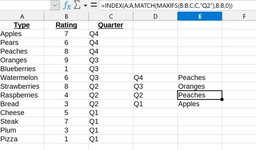
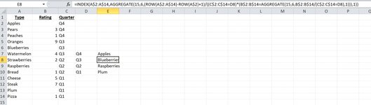
What I'm trying to do. I want a formula to return text from Column A based on the highest number in Column B, but only in cells that match Column C.
I've attached a photo.
Essentially I only want the highest result for each quarter.
In the example I listed above, this works for Q4 and Q3 but not for Q2 and Q1. The photo has the formula for Q2 but I'll post it here as well:
=INDEX(A:A,MATCH(MAXIFS(B:B,C:C,"Q2"),B:B,0))
The formulas are all the same, just the "Q#" is changed.
What it's doing is searching based on the criteria but then giving me the first result with criteria ignored. So for Q2 it sees that "Strawberries" with an 8 is the highest, but then it spits out "Peaches" as that's the first 8 in the column, even though I told it only ones that match Q2.
Please let me know what I'm doing wrong and what I can do to achieve what I need.
Thanks!
I'll explain what I'm trying to do then tell you what I'm currently doing that isn't working as I want it to.
What I'm trying to do. I want a formula to return text from Column A based on the highest number in Column B, but only in cells that match Column C.
I've attached a photo.
Essentially I only want the highest result for each quarter.
In the example I listed above, this works for Q4 and Q3 but not for Q2 and Q1. The photo has the formula for Q2 but I'll post it here as well:
=INDEX(A:A,MATCH(MAXIFS(B:B,C:C,"Q2"),B:B,0))
The formulas are all the same, just the "Q#" is changed.
What it's doing is searching based on the criteria but then giving me the first result with criteria ignored. So for Q2 it sees that "Strawberries" with an 8 is the highest, but then it spits out "Peaches" as that's the first 8 in the column, even though I told it only ones that match Q2.
Please let me know what I'm doing wrong and what I can do to achieve what I need.
Thanks!