Index match multi criteria - help

[tonyotter]

Dear Mr Excel Community,

Hoping once again for you to come to my rescue

I am looking for some help on trying to solve the following index match problem (Although it may be solve with a solution that isn't index/match)
I have tried a number of solutions both array and non-array but with no luck so far.

I have the following in sheet1:
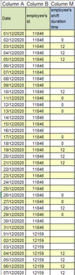
In Colum A are dates beginning 1st December (a2) through to 31st (a32)
In Column B is an employee payroll number (e.g. 11846) the same number through cells B2 to B32
In Column M are values showing the hours worked by the employee on that day (Value can be blank / zero or any number - 2 decimals up to 18)

This pattern then repeats for the subsequent rows with the next employee payroll number - i.e. A33 through to A63 will be dates 1st to 31st again, whilst B33 through B63 will be the next employee ID number.
The pattern runs through all employee ID numbers.

In sheet 2

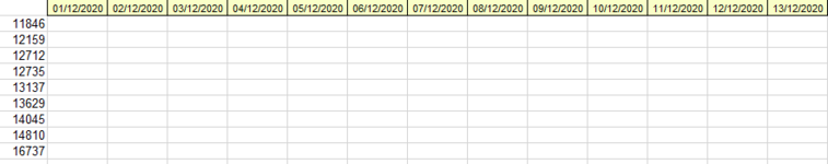
I have in column A all unique employee ID numbers starting at A2.
In Row 1 I have dates from the first of December (B1) through to 31st December (AF1)

What I need to achieve is in each row next to the unique ID number to lookup the ID number in sheet 1 and the corresponding date in sheet1 and return the hours in column M

Example result to be generated attached.

I hope I have been clear - I have tried various ways as detailed in posts here and elsewhere but cannot get this to work.

Greatly appreciate any help

 

[Fluff]

I suggest that you update your Account details (click your user name at the top right of the forum) so helpers always know what Excel version(s) & platform(s) you are using as the best solution often varies by version. (Don’t forget to scroll down & ‘Save’)

How about, in B2 dragged down & across

=SUMIFS(Sheet1!$M:$M,Sheet1!$B:$B,$A2,Sheet1!$A:$A,B$1)