Index/Match multiple hits of same cell value and add rows to fit spill

[kidneythief]

Hi guys! Not sure how to approach this - with lookup and aggregate, an index/match sub or something else.

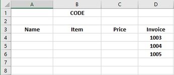
So In the sheet called Empty, when B2 is filled, it populates the Invoice column in D4:D with unique invoice numbers from an external order sheet.
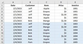
The Sales sheet has a list of orders where each invoice is broken down per item (so each single invoice number in the Empty sheet can have multiple instances
in the Sales sheet).

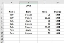
I need to pull data from the Sales sheet into the Empty sheet using the invoice numbers as a reference. However, since the Empty sheet only pulls a single
instance of each invoice number, I need to manage spillover and insert rows when needed, as seen in the Filled sheet.

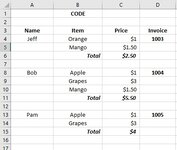
Going further, I was wondering if it would be possible to transpose output into something like what's shown in the Filled_Alt sheet, where Name and Invoice
(A2 and D2) are not repeated, and an extra row is added where the Price column items (or any additonal columns added there like quantity, etc.) are added up.

Ideally, the whole sheet would be populated as in Filled_Alt automatically each time B2 is changed and a new set of invoice numbers populate the D column.

Sorry to be asking so much, and I'd be really grateful for any help or guidance on this.

 

[jasonb75]

If that is now showing your actual layout then I think that a whole new approach will be required. The Orders sheet in the file linked to post 7 is in a format that will work with formulas, the layout that is shown in the TripSheet image in post 10 is too disorganised to work with formulas.

In my opinion, either the TripSheet needs to be better organised so that it resembles the format of the Orders sheet in the earlier attachment so that formulas can be used, or a vba method will be needed instead. Unfortunately the latter is not something that I would be able to help you with at the moment. Hopefully another member of the forum will pick up on your unsolved question and be able to assist you with the vba method if you choose that option.

 

[kidneythief]

If that is now showing your actual layout then I think that a whole new approach will be required. The Orders sheet in the file linked to post 7 is in a format that will work with formulas, the layout that is shown in the TripSheet image in post 10 is too disorganised to work with formulas.

In my opinion, either the TripSheet needs to be better organised so that it resembles the format of the Orders sheet in the earlier attachment so that formulas can be used, or a vba method will be needed instead. Unfortunately the latter is not something that I would be able to help you with at the moment. Hopefully another member of the forum will pick up on your unsolved question and be able to assist you with the vba method if you choose that option.

Yeah, I understand, it's been really hard working with set layouts that I'm not allowed to change, particularly the TripSheet. I do have a vba that pulls the relevant invoices from the TripSheet
into the Output sheet so that it resembles something like the Empty sheet from the original post. If I have the unique invoices in the Output sheet, is there some way to pull all their instances from the Sales sheet using formulas?

 

[fjns]

Hi, I created the newer version of the table based on your #10 message.

MultipleNewer.xlsx

 

[kidneythief]

Hi, I created the newer version of the table based on your #10 message.

MultipleNewer.xlsx

Hi fjns! Thank you, the output in the FilledSums sheet comes out perfect! I was wondering, is it possible to merge the first three sheets (empty, filled, and FilledSums) or remove the first
two so that I can just input date and truck selections in the FilledSums sheet and get the same result? Also, does Array Constrain only work in Google Sheets? (This isn't really a problem
if that's the case as I can inform the user to just use GSheets). This is a lot to go over for me but I'll spend the next day or so trying to understand the formulas myself! For now I'd like to
mark this as the solution but I hope you don't mind if I have a few questions about your formulas! Again, thank you for your time

 

[fjns]

Hi, I am very glad that the formulas work.
If I have enough knowledge, I am happy to help at any time.

 

[kidneythief]

Hi, I am very glad that the formulas work.
If I have enough knowledge, I am happy to help at any time.

Hi fjns! I had a question about the formulas. In the FilledSums sheet, it seems in the datasets I will be using, there are so many invoice numbers used that some new booklets overlap but with a zero at the start. For instance, there can be an SI# 1001 and a different one that is SI# 01001. The problem, I think, is that the formula grabs both numbers even if the date or tripsheet codes are different. Sorry, I really don't know which part of the formula you made I should change to fix this. I'd be grateful for any help with this!

 

[fjns]

Hi, the correct functioning of SI# 1001 and SI# 01001 requires changing the formatting of 7 columns from General to Text. All formulas in the table are unchanged.
The 7 columns:
Empty!G (SI#)
Filled!G (SI#)
FilledSums!G (SI#)
tech!G (AuxC7)
tech!Y (AuxC23)
Sales!G (Invoice#)
TripSheet!G (Invoice#)

MultipleNewer2.xlsx

 

[kidneythief]

Hi, the correct functioning of SI# 1001 and SI# 01001 requires changing the formatting of 7 columns from General to Text. All formulas in the table are unchanged.
The 7 columns:
Empty!G (SI#)
Filled!G (SI#)
FilledSums!G (SI#)
tech!G (AuxC7)
tech!Y (AuxC23)
Sales!G (Invoice#)
TripSheet!G (Invoice#)

MultipleNewer2.xlsx

I actually already tried this, but it seems if the invoice number starting with zero is on another TripSheet block, it still pops up. For example, in your worksheet,
if I instead replace the 1009 invoice with 01001, the 01001 invoice number still appears along with 1001.

 

[fjns]

Hi, I created a new table.

The new formulas used in the new table:
Filled!G7: =IF(ROW()>tech!H$2,"",SUBSTITUTE(INDEX(tech!G:G,MATCH(ROW(),tech!J:J,0)),"#",""))
FilledSums!G7: =LET(i,IFERROR(MATCH(ROW(),tech!N:N,0),0),IF(ROW()>tech!K$2,"",IF(i=0,"",IF(INDEX(tech!L:L,i)=1,SUBSTITUTE(INDEX(tech!G:G,i),"#",""),""))))
tech!G2: =IF(OR(INDEX(Sales!A:A,ROW())="",INDEX(Sales!B:B,ROW())="",INDEX(Sales!G:G,ROW())=""),"","#"&INDEX(Sales!G:G,ROW()))
tech!Y2: =LET(x,INDEX(TripSheet!A:A,ROW()),y,"#"&INDEX(TripSheet!C:C,ROW()),IF(OR(x="",y=""),"",IF(IFERROR(SEARCH("--- ",x),0)>0,"",y)))

The formatting

General:
Empty!G (SI#)
Filled!G (SI#)
FilledSums!G (SI#)
tech!G (AuxC7)
tech!Y (AuxC23)

Text:
Sales!G (Invoice#)
TripSheet!G (Invoice#)

MultipleNewer3.xlsx

 

[kidneythief]

Hi, I created a new table.

The new formulas used in the new table:
Filled!G7: =IF(ROW()>tech!H$2,"",SUBSTITUTE(INDEX(tech!G:G,MATCH(ROW(),tech!J:J,0)),"#",""))
FilledSums!G7: =LET(i,IFERROR(MATCH(ROW(),tech!N:N,0),0),IF(ROW()>tech!K$2,"",IF(i=0,"",IF(INDEX(tech!L:L,i)=1,SUBSTITUTE(INDEX(tech!G:G,i),"#",""),""))))
tech!G2: =IF(OR(INDEX(Sales!A:A,ROW())="",INDEX(Sales!B:B,ROW())="",INDEX(Sales!G:G,ROW())=""),"","#"&INDEX(Sales!G:G,ROW()))
tech!Y2: =LET(x,INDEX(TripSheet!A:A,ROW()),y,"#"&INDEX(TripSheet!C:C,ROW()),IF(OR(x="",y=""),"",IF(IFERROR(SEARCH("--- ",x),0)>0,"",y)))

The formatting

General:
Empty!G (SI#)
Filled!G (SI#)
FilledSums!G (SI#)
tech!G (AuxC7)
tech!Y (AuxC23)

Text:
Sales!G (Invoice#)
TripSheet!G (Invoice#)

MultipleNewer3.xlsx

should I still enter those as arrays or enter as is?