Index Match not working.

[CaptainPP]

Hi everyone.
I am pretty new to excel but have been doing ok often due to help from MrExcel members.
I am trying to return a number based on two criteria using the following array formula.
=INDEX($D$2:$D$2000,MATCH($A2,$D2:$D$2000,0)*MATCH($L$2,$I$2:$I$2000,0))
I have entered it using shift and ctrl but it doesn't work, i get #N/A or 0 but not the return from column D that i want.
Hopefully something silly will be obvious to one of you and i can fix it quickly.
Thanks in advance.
Paul

 

[jasonb75]

You can't multiply matches, that is a recipe for disaster.
Here's one way that works. If column D contains numbers / dates then it can be shortened a bit. This version works with numbers or text.

=INDEX($D:$D,AGGREGATE(16,6,ROW($D$2:$D$2000)/($D2:$D$2000=$A2)/($I$2:$I$2000=$L$2),1))

 

[Toadstool]

@jasonb75 Can you explain the use of the AGGREGATE 16 function number? I assume it's a typo.

Hi CaptainPP,

I'm not sure what you're trying to achieve. If both of your MATCH functions find a match then the two row numbers where they matched will be multiplied together, which will often access an unused column D cell so return a zero.

In your formula $A2 is relative so will the formula be copied down?
In your formula $L$2 and $I$2 are absolute so does $L$2 just need to appear anywhere in column I or does it need to be the same row as when A matches D?

Maybe you can explain further or better give an example?

Here I've made a small change to your formula which gives a result, though probably not what you want.

CaptainPP.xlsx
	A	B	C	D	E	F	G	H	I	J	K	L	M	N
1	ColA			ColD					ColI			ColL		CaptainPP
2	4			3					Mouse			Goat		4
3	6			2					Mole					#N/A
4	3			4					Cat					3
5	2			3					Goat					2
6	5			5					Horse					5
7	4			4					Goat					4
8	7			7										7
9	2			2										2
10
Sheet1

Cell Formulas
Range	Formula
N2:N9	N2	=INDEX($D$2:$D$2000,MATCH($A2,$D$2:$D$2000,0)*ISNUMBER(MATCH($L$2,$I$2:$I$2000,0)))

 

[jasonb75]

@jasonb75 Can you explain the use of the AGGREGATE 16 function number? I assume it's a typo.

yeah, should have been 15.

I would advise against your method though, as I said in my post, multiplying matches is a recipe for disaster. (note that I've only CSE entered the formula to stop it from spilling in 365).

Book1
	A			D					I			L		N
1	ColA			ColD					ColI			ColL		CaptainPP
2	4			3					Mouse			cheese		3
3	6			2					Mole					#N/A
4	3			4					Cat					3
5	2			3					Goat					3
6	5			5					Horse					3
7	4			4					Goat					3
8	7			7										3
9	2			2
Sheet20

Cell Formulas
Range	Formula
N2:N8	N2	=INDEX($D$2:$D$2000,MATCH($A2,$D$2:$D$2000,0)*ISNUMBER(MATCH($L$2,$I$2:$I$2000,0)))
Press CTRL+SHIFT+ENTER to enter array formulas.

 

[CaptainPP]

Thanks for the replies.
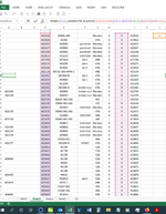
I will try to explain what i am doing a little better. I want to return the value from column A only if it matches a number in column D and a number ($L$2 could change to 1 as this is always the required number) in column I.
I will attach a screen shot of the current set up as i may be overcomplicating things.

 

[bebo021999]

Look like you want to extract a list from D column, with corresponding 1 in column I, and must be found in column A?

TABEL EXAMPLE.xlsx
	A	B	C	D	E	F	G	H	I	J	K	L	M	N
1														List of value from D that match A
2	421			421					0			1		423
3	423			422					0					425
4				423					1
5	425			424					0
6				425					1
7	426			426					0
8				427					0
9				428					0
10				429					0
11				430					0
12				431					0
13				432					0
Sheet3

Cell Formulas
Range	Formula
N2:N10	N2	=IFERROR(INDEX(D:D,AGGREGATE(15,6,ROW($A$2:$A$13)/(COUNTIF($A$2:$A$13,$D$2:$D$13)=1)/($I$2:$I$13=$L$2),ROW(1:1))),"")

 

[CaptainPP]

Exactly right bebo021999.
I was expecting the number in A to be reproduced opposite the original but your table of results is great.
I don't understand aggregate in excel (or many other things in excel to be honest) but your formula is working fine now so i will worry about that later!
Thanks for your help everyone.

 

[jasonb75]

With numeric results, you don't need the INDEX function and can shorten the formula to

=IFERROR(AGGREGATE(15,6,$D$2:$D$13/(COUNTIF($A$2:$A$13,$D$2:$D$13)=1)/($I$2:$I$13=$L$2),ROWS(N$2:N2)),"")

Also, I've changed ROW(1:1) to ROWS(N$2:N2) which is the cell that holds the first formula in the table. Using ROW(1:1) can cause the formula to fail if you insert or delete rows.

Finally, if duplicates in column A are possible then you might need to change =1 to >=1, or something else entirely depending on the expected results,

 

[bebo021999]

With numeric results, you don't need the INDEX function and can shorten the formula to

=IFERROR(AGGREGATE(15,6,$D$2:$D$13/(COUNTIF($A$2:$A$13,$D$2:$D$13)=1)/($I$2:$I$13=$L$2),ROWS(N$2:N2)),"")

Also, I've changed ROW(1:1) to ROWS(N$2:N2) which is the cell that holds the first formula in the table. Using ROW(1:1) can cause the formula to fail if you insert or delete rows.

Finally, if duplicates in column A are possible then you might need to change =1 to >=1, or something else entirely depending on the expected results,

Thanks. You are right by changing ROW to ROWS
BTW, the OP did not mention column D is increasing order, though it appears to be. If it is, yours is correct with A-Z sorting list. If it is not, not sure a sorting list meets his requirement.

 

[CaptainPP]

Both answers are working well thanks guys. You are right that column D is always in ascending order bebo021999 and there will never be duplicates in A jasonb75 so all good.