Index/match or vlookup a range where value matches in a table

[cderhay]

I have been trying to figure out how to utilize a simple index/match, or even vlookup to return the value that is in that column and matches the same Team ID.

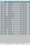
I have a table that has different team IDs is column A, and 3 different point values in column D. depending on the points, is the dollar amount. I want it to look up the dollar amount for the point values of the team ID that matches item.

I want to return the dollar amount listed in Levels[Agent} based on how many points were obtained (G2) will fall into 1 of 3 tiers in Levels[Total Points Range]

=INDEX(Levels[Agent],MATCH(G2,Levels[Total Points Range]))
=VLOOKUP(G2,Levels[Total Points Range]:Levels[Agent],2,TRUE)

BUT ALSO the Levels[Agent] amount that matches the Team ID (Column A) with the Team ID in Levels[Team]

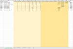
below is the closest i have got, but it doesn't work as row 8 should not be returning any value as there is no amount listed in the Levels[Agent} column for that team

=INDEX(Levels[Agent],MATCH(A2&G2,Levels[Team]&Levels[Total Points Range]))

Please help!!!

 

[jasonb75]

You're using approximate match, not exact match. This means that when there is no exact match the closest match (less than the exact match) is returned instead.

To only get exact matches, you need to use

=INDEX(Levels[Agent],MATCH(A2&G2,Levels[Team]&Levels[Total Points Range],0))

This will show an error when there is no match, so you would need to use an error trap to keep your sheet tidy.

=IFERROR(INDEX(Levels[Agent],MATCH(A2&G2,Levels[Team]&Levels[Total Points Range],0)),"")

 

[cderhay]

thank you!!!

Unfortunately that is part of my dilemma. The approximate match was due to the fact that the points will fall in 1 of 3 tiers, and will not match exactly. That's the trouble i seem to have. how do i match exact the team, then look for the tier?

 

[jasonb75]

Now I see the problem, as the result is a numeric (cash) value, I would suggest using a totally different method.

=MAXIFS(Levels[Agent],Levels[Team],A2,Levels[Total Points Range],"<="&G2)

edit:-

If that doesn't do what you need, then you could try

=INDEX(Levels[Agent],MATCH(A2&LOOKUP(G2,{0,10,30}),Levels[Team]&Levels[Total Points Range],0))

 

[cderhay]

that second one looks like it worked well!!! thank you so much!! this about drove me nuts