Index Match returns #n/a on some cells and not others! driving me crazy!

[dhune]

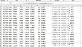
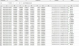
Hi, i'm currently using index match to retrieve values from an array with 50000 rows. My problem is with the match lookup value and array part. The lookup value is a date with dd/mm/yy hh:mm format and the lookup array is in the same format (column J and A). I can't upload a mini sheet as the first column A has 50000 rows and if I just cut the first few rows at the top, it won't work because the values I want to lookup are thousands of rows down in column A, so I hope the pictures will make sense.

In column J where I have my lookup values, I have different dates with similar times of the day (hh:mm). Now, I want to retrieve the values from column G into column K so i have the formula =INDEX($G$1:$G$50000,MATCH(J1,$A$1:$A$50000,0)). I copied the values in column I from a different source which has different dates but with similar times (either 8:30:00 or 9:30:00 am). I want to retrieve values from column G corresponding to the dates in column J but with times 8:45 am and 9:45 am (not 8:30 am and 9:30 am) so I just added 15 minutes to the values in column I and I have this formula in column J =I1+TIME(0,15,0). The weird thing is the index match formula returns values in column K but only on the rows where the corresponding times are at 9:45 and then returns #N/A in the cells with corresponding times at 8:45 am! I checked the formatting on column A and J to make sure they are the same and also pressed ctrl+shift+enter after completing the index match formula in column K. The puzzling thing is, if I delete cell J1 and type the date and time MANUALLY instead of using the formula J1=I1+TIME(0,15,0) to get 8:45 am, the index match formula returns a value! I've tried copy pasting column J as values to remove the formulas but to no avail. I still get #N/A for the 8:45 times. The values do exist in column A, that is for sure, I checked them manually. I don't get why the formula would work on the cells where the corresponding time I want to retrieve from is at 9:45am and not those where the time is 8:45am...

I did copy the values in column I from an internet page then pasted them in excel, not sure if this would be causing my problem?

 

[mart37]

Why are you using an array-formula?
Use column A seconds?
You can set the format of column A to number. Then you can compare with column J (also set to number). Control the numbers behind the comma.

 

[mart37]

Maybe you need to convert column A: =INT(A1)+TIME(HOUR(A1),MINUTE(A1),0)

 

[joeu2004]

I can't upload a mini sheet as the first column A has 50000 rows

Using XL2BB to include even the first few of many similar rows can be helpful because it shows your exact formulas. That said, you did a good job of the alternative, presenting and explaining repetitive formulas.

pressed ctrl+shift+enter after completing the index match formula in column K

I see no reason to array-enter that formula. Although there is no harm, it is better not to. It makes it easier to edit.

I have this formula in column J =I1+TIME(0,15,0)

You are probably encountering problems with 64-bit binary floating-point arithmetic.

In general, whenever we need a calculation to be accurate to some degree of precision (decimal places or, in this case, minutes or seconds), we should explicitly round to that degree of precision -- and not to arbitrary number of decimal places like 10, as some people suggest.

Change the calculation in column J to something like the following to round to the minute:

=INT(I1+TIME(0,15,0)) + TEXT(I1+TIME(0,15,0), "h:m")

Likewise, I suspect that column A should be populated with formulas of the following form:

=INT(A1+TIME(0,15,0)) + TEXT(A1+TIME(0,15,0), "h:m")

The INT part captures the date part without relying on the regional date format, which might vary if you share the workbook.

To demonstrate:

book1.xls
	A	B	C	D
1	3/6/2021 8:30		internal value	residual
2	3/6/2021 8:45		44261.3645833333	3.63798E-11
3	3/6/2021 8:45	FALSE	44261.3645833333	2.91038E-11
4	3/6/2021 8:45	TRUE	44261.3645833333	3.63798E-11
Sheet2

Select or hover the cursor over cells to see formulas.

Column C shows the internal numeric value of the date/times in column A, formatted to display 15 significant digits, the most that Excel formats. Column D shows the invisible residual offset, effectively the additional precision that Excel does not display. Note the difference between A3 and A2; and note that A4 and A2 are identical.

 

[dhune]

Using XL2BB to include even the first few of many similar rows can be helpful because it shows your exact formulas. That said, you did a good job of the alternative, presenting and explaining repetitive formulas.



I see no reason to array-enter that formula. Although there is no harm, it is better not to. It makes it easier to edit.



You are probably encountering problems with 64-bit binary floating-point arithmetic.

In general, whenever we need a calculation to be accurate to some degree of precision (decimal places or, in this case, minutes or seconds), we should explicitly round to that degree of precision -- and not to arbitrary number of decimal places like 10, as some people suggest.

Change the calculation in column J to something like the following to round to the minute:

=INT(I1+TIME(0,15,0)) + TEXT(I1+TIME(0,15,0), "h:m")

Likewise, I suspect that column A should be populated with formulas of the following form:

=INT(A1+TIME(0,15,0)) + TEXT(A1+TIME(0,15,0), "h:m")

The INT part captures the date part without relying on the regional date format, which might vary if you share the workbook.

To demonstrate:

book1.xls
	A	B	C	D
1	3/6/2021 8:30		internal value	residual
2	3/6/2021 8:45		44261.3645833333	3.63798E-11
3	3/6/2021 8:45	FALSE	44261.3645833333	2.91038E-11
4	3/6/2021 8:45	TRUE	44261.3645833333	3.63798E-11
Sheet2

Select or hover the cursor over cells to see formulas.

Column C shows the internal numeric value of the date/times in column A, formatted to display 15 significant digits, the most that Excel formats. Column D shows the invisible residual offset, effectively the additional precision that Excel does not display. Note the difference between A3 and A2; and note that A4 and A2 are identical.

Awesome! That did it! You sir (or ma'am) just saved my sanity. Thank you very much.

 

[dhune]

Maybe you need to convert column A: =INT(A1)+TIME(HOUR(A1),MINUTE(A1),0)

Thank you very much! This did the trick!