index match with multiple criteria

[vkorla]

Hello! I'd like to create a formula that, given a particular value for "Age" and "Education", returns the mean and standard deviation from another table. The raw data are in the "Raw data" image file attached, and the values for the mean and standard deviation are in the "Mean st dev" image file, also attached.

For example if I need to find the mean and standard deviation of Age = 23, and Education = 6, the correct values that should be returned are:
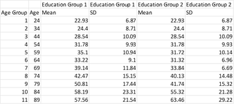
Mean = 22.93 (because age = 23 is in age group 1)
Standard deviation = 6.87 (because education = 6 is in education group 1)

How can I best achieve this so that I can input any values for age and education to get the correct mean & standard deviation values?

Thanks so much!

 

[Leo Skywalker]

Try this:

Book3
	A	B	C	D	E	F	G	H	I	J	K	L
1
2							Age	35		Mean	KK
3	Age	Age Group		Education	Ed Group		Education	29		StDev	LL
4	18	1		1	1
5	19	1		2	1
6	20	1		3	1
7	21	1		4	1
8	22	1		5	1
9	23	1		6	1
10	24	1		7	1				ED GROUP 1		ED GROUP 2
11	25	2		8	1		Age Group	Age	Mean	SD	Mean	SD
12	26	2		9	1		1	24	AA	BB	CC	DD
13	27	2		10	1		2	34	EE	FF	GG	HH
14	28	2		11	1		3	44	II	JJ	KK	LL
15	29	2		12	2		4	54	100	200	300	400
16	30	2		13	2		5	59	500	600	700	800
17	31	2		14	2		6	64	a	f	j	n
18	32	2		15	2		7	69	b	g	k	o
19	33	2		16	2		8	74	c	h	l	p
20	34	2		17	2		9	79	OO	PP	QQ	RR
21	35	3		18	2		10	84	SS	TT	UU	VV
22	36	3		19	2		11	89	WW	XX	YY	ZZ
23	37	3		20	2
24	38	3		21	2
25	39	3		22	2
26	40	3		23	2
27	41	3		24	2
28	42	3		25	2
29	43	3		26	2
30	44	3		27	2
31	45	4		28	2
32	46	4		29	2
33	47	4		30	2
34	48	4
35	49	4
36	50	4
37	51	4
38	52	4
39	53	4
40	54	4
41	55	5
42	56	5
43	57	5
44	58	5
45	59	5
46	60	6
47	61	6
48	62	6
49	63	6
50	64	6
51	65	7
52	66	7
53	67	7
54	68	7
55	69	7
56	70	8
57	71	8
58	72	8
59	73	8
60	74	8
61	75	9
62	76	9
63	77	9
64	78	9
65	79	9
66	80	10
67	81	10
68	82	10
69	83	10
70	84	10
71	85	11
72	86	11
73	87	11
74	88	11
75	89	11
Sheet2

Cell Formulas
Range	Formula
K2	K2	=INDEX(I$12:L$22,VLOOKUP($H$2,A3:B75,2,0),INT(1.5*(VLOOKUP($H$3,$D$3:$E$33,2,0))))
K3	K3	=INDEX(I$12:L$22,VLOOKUP($H$2,A4:B76,2,0),INT(2*(VLOOKUP($H$3,$D$3:$E$33,2,0))))

 

[vkorla]

This is perfect, thanks so much Leo Skywalker! Question, why are you using the INT function?

 

[Leo Skywalker]

This is perfect, thanks so much Leo Skywalker!

Glad to help!, if the post is the solution, please mark it as solved.

why are you using the INT function?

in K1, It's just a way to convert education type 1 and 2 to 1 and 3, to select the appropriate colums for the VLOOKUP.
int(1x1.5)=1
int(2x1.5)=3
There are other ways to get the same result, for example:
2n-1 then:
(1x2)-1=1
(2x2)-1=3

In K2, it's not needed,
1x2=2
2x2=4 they are already intergers, I just didn't delete for lazyness.