Hello,
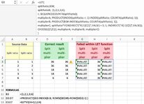
I'm calculating Split Multiplier column from Split Ratio column by multiplying the rows from the current row towards the end of the column. It works nicely within normal excel table with PRODUCT($B3:INDEX(B:B; ROWS($B$3#)+ROW($B$3)-1) ) where the formula is copied down, but if I try to apply this within LET-function I just get #VALUE error.
The other solution I have tried gives the same error:If replace B3*IF(E4=0;1;E4) with multiplierC; splitRatio*IF(INDIRECT("R[-1]C[1]";FALSE) = 0; 1; INDIRECT("R[-1]C[1]";FALSE));
In this latter case, it looks like that there are no way to refer to the column that I'm currently calculating. Is that a case?
See my excel sheet and formulas in the attached picture.
I'm wondering if I am trying to achieve something that LET function cannot handle?