Insert customer to worksheet then sort

[ipbr21054]

Morning,
I am using the code shown below.

I enter details on my userform then pressing the command button sends those details to my worksheet & sorts column A-Z

A couple of times now it doesnt sort.
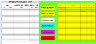
Ive just added a new customer for which is M HOUSE G + S.
It should of been sorted so its at N23 but its last at N32

Can you see an issue in the code.
My current worksheet where the details are stored is N4 - R32

Private Sub CommandButton1_Click()
    Dim i           As Integer
    Dim LastRow     As Long
    Dim wsGIncome   As Worksheet
    Dim arr(1 To 5) As Variant
    Dim Prompt      As String
  
    Set wsGIncome = ThisWorkbook.Worksheets("G INCOME")
  
    For i = 1 To 5
        Prompt = Choose(i, "CUSTOMERS'S NAME", "ADDRESS", "POST CODE", "CHARGE", "MILEAGE")
        With Me.Controls("TextBox" & i)
            If Len(.Value) = 0 Then
                MsgBox "NO " & Prompt & " & WAS ENTERED", 16, Prompt & " Empty MESSAGE"
                .SetFocus
                Exit Sub
            Else
                If InStr(1, .Value, "£") = 1 Then
                    arr(i) = CCur(.Value)
                ElseIf IsDate(.Value) Then
                    arr(i) = DateValue(.Value)
                ElseIf IsNumeric(.Value) Then
                    arr(i) = Val(.Value)
                Else
                    arr(i) = .Value
                End If
            End If
          
        End With
    Next i
      
         Application.ScreenUpdating = False
        With wsGIncome
            LastRow = .Cells(.Rows.Count, "N").End(xlUp).Row + 1
          
            With .Cells(LastRow, 14).Resize(, UBound(arr))
                .Value = arr
                .Font.Name = "Calibri"
                .Font.Size = 11
                .Font.Bold = True
                .HorizontalAlignment = xlCenter
                .VerticalAlignment = xlCenter
                .Borders.Weight = xlThin
                .Interior.ColorIndex = 6
            End With
          
          
            .Cells(LastRow, "N").HorizontalAlignment = xlLeft
         
          
            If .AutoFilterMode Then .AutoFilterMode = False
            x = .Cells(Rows.Count, 4).End(xlUp).Row
            .Range("N4:R" & x).Sort Key1:=.Range("N4"), Order1:=xlAscending, Header:=xlGuess
         
            .Range("N4").Select
          
        End With

       Unload Me
        Application.ScreenUpdating = True
         MsgBox "DATABASE SUCCESSFULLY UPDATED", vbInformation, "GRASS INCOME NAME & ADDRESS MESSAGE"

    End Sub

 

[johnnyL]

Just taking a stab here but maybe replace:

.Range("N4:R" & x).Sort Key1:=.Range("N4"), Order1:=xlAscending, Header:=xlGuess

With:

.Range("N4:R" & x).Sort Key1:=.Range("N4"), Order1:=xlAscending, Header:=xlGuess, Orientation:=xlSortColumns

 

[ipbr21054]

Many thanks but that didnt work but i have found why its happening now but advice is still required.

On the left of the worksheet i have a summary of which in cell D31 is Autosum for D5-D30 & in cell E31 i have Autosum for E5-E30
Now on the right is my vlookup section with names, address etc.
Currently when filled in the last row is 31
So both are on row 31

On my vlookup section the A-Z sort doesnt happen after the row 31 BUT if i enter a value in cells D32 & E32 then add tpo the vlookup it then works fine.
Same again after that in respect of the row ????

 

[ipbr21054]

Following on from above.
The values on the right will only work correctly IF a valve is in column cells D

Currently the last value in column D is at row 31 so the last correctly sorted value on the right will be 1 row down thus being row 32
This has a pattern down the page.

If cell D32 is empty then the sort on the right will not happen.
BUT if i put a value in cell D32 then the sort works and the last row with a value in will be 1 row down thus row 33

Some other info if needed.
Cell C5 and down the page is =IFERROR(VLOOKUP($B5,$N:$DC,2,FALSE),"")

Cell D5 and down the page is =IFERROR(VLOOKUP($B5,$N:$DC,4,FALSE),"

Cell E5 and down the page is =IFERROR(VLOOKUP($B5,$N:$DC,5,FALSE),"")

Selecting a cell in column B then gpoing to Data / Data Validation i see Source=GRASSTABLE

Selecting Formulas / Name Manager i see GRASSTABLE referes to =OFFSET('G INCOME'!#REF!,0,0,COUNTA('G INCOME'!$N:$N),1)

One thing i have noticed is that the above line of code now shows #REF where before it would show =OFFSET('G INCOME'!$N$4,0,0,COUNTA('G INCOME'!$N:$N),1)

So why has that changed ?

Thanks for your time