Is there a regional settings issue in this formula?

[valmir]

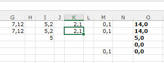
The formula in column O is not behaving the way it is supposed to. Can someone please check and be able to tell me why it is not working for me? The formula is supposed to sum the whole part and the decimal part of the number separately and then present the result separated by a comma. Somehow, when I try it, it is not showing the decimal parts of the sum. Please help!

ztest3.xlsx
	G	H	I	J	K	L	M	N	O
1	7,12		5,2		2,1		0,1		14,0
2	7,12		5,2		2,1		0,1		14,0
3			5						5,0
4									0,0
5							0,1		0,0
Sheet1

Cell Formulas
Range	Formula
O1:O5	O1	=(TRUNC(G1,0)+TRUNC(I1,0)+TRUNC(K1,0)+TRUNC(M1,0))&","&IFERROR(VALUE(MID(G1-TRUNC(G1,0),FIND(".",G1-TRUNC(G1,0))+1,256)),0)+IFERROR(VALUE(MID(I1-TRUNC(I1,0),FIND(".",I1-TRUNC(I1,0))+1,256)),0)+IFERROR(VALUE(MID(K1-TRUNC(K1,0),FIND(".",K1-TRUNC(K1,0))+1,256)),0)+IFERROR(VALUE(MID(M1-TRUNC(M1),FIND(".",M1-TRUNC(M1))+1,256)),0)

Cells with Conditional Formatting
Cell	Condition		Cell Format	Stop If True
G1:N2,O1:P5	Cell Value	=0	text	NO

This is what I'm getting:

 

[jasonb75]

What results should you be getting? The way that you describe the problem says that you only need to use a simple =SUM(G1:M1) formula in place of what you have.

The only reason I can see for using a formula like that would be if you are trying to use comma decimals with period decimal system settings.

Copying your mini sheet to my laptop (period decimal settings) produces these results, are they correct?
I would have thought that the first 2 rows should be 14,52 not 14,16 as the formula returns.

Book1
	G	H	I	J	K	L	M	N	O
1	7.12		5.2		2.1		0.1		14,16
2	7.12		5.2		2.1		0.1		14,16
3			5						5,0
4									0,0
5							0.1		0,1
Sheet15

Cell Formulas
Range	Formula
O1:O5	O1	=(TRUNC(G1,0)+TRUNC(I1,0)+TRUNC(K1,0)+TRUNC(M1,0))&","&IFERROR(VALUE(MID(G1-TRUNC(G1,0),FIND(".",G1-TRUNC(G1,0))+1,256)),0)+IFERROR(VALUE(MID(I1-TRUNC(I1,0),FIND(".",I1-TRUNC(I1,0))+1,256)),0)+IFERROR(VALUE(MID(K1-TRUNC(K1,0),FIND(".",K1-TRUNC(K1,0))+1,256)),0)+IFERROR(VALUE(MID(M1-TRUNC(M1),FIND(".",M1-TRUNC(M1))+1,256)),0)

 

[valmir]

What results should you be getting? The way that you describe the problem says that you only need to use a simple =SUM(G1:M1) formula in place of what you have.

The only reason I can see for using a formula like that would be if you are trying to use comma decimals with period decimal system settings.

Copying your mini sheet to my laptop (period decimal settings) produces these results, are they correct?
I would have thought that the first 2 rows should be 14,52 not 14,16 as the formula returns.

Book1
	G	H	I	J	K	L	M	N	O
1	7.12		5.2		2.1		0.1		14,16
2	7.12		5.2		2.1		0.1		14,16
3			5						5,0
4									0,0
5							0.1		0,1
Sheet15

Cell Formulas
Range	Formula
O1:O5	O1	=(TRUNC(G1,0)+TRUNC(I1,0)+TRUNC(K1,0)+TRUNC(M1,0))&","&IFERROR(VALUE(MID(G1-TRUNC(G1,0),FIND(".",G1-TRUNC(G1,0))+1,256)),0)+IFERROR(VALUE(MID(I1-TRUNC(I1,0),FIND(".",I1-TRUNC(I1,0))+1,256)),0)+IFERROR(VALUE(MID(K1-TRUNC(K1,0),FIND(".",K1-TRUNC(K1,0))+1,256)),0)+IFERROR(VALUE(MID(M1-TRUNC(M1),FIND(".",M1-TRUNC(M1))+1,256)),0)

Hi Jason! The results that you just published is exactly the intended result but somehow, I am getting the results as on the image. Yes, I know that in the conventional way, the results should be 14,52 etc etc but as I explained, I want each part of the decimal number summed separately and then each part shown separated by a comma. I've been told by someone else that this formula is right. I'm just wondering why in my case, it is not summing the "decimal" part of the number. The image that I posted is what I am getting when I copy paste down the formula. Is it because the formula was designed to be used by dots as opposed to commas due to my regional settings? Anyway, I found the solution myself and the solution was right there in my title. All I had to do is change the "." into "," exactly because of "regional settings" as I suspected!

 

[jasonb75]

Is it because the formula was designed to be used by dots as opposed to commas due to my regional settings?

It would certainly seem that way. Now that I understand exactly what you want it to, I'll have another look and see what it needs to make it work.

 

[valmir]

ok and I have another question. Can it be made to behave as a number or it will have to behave as text?

 

[jasonb75]

See if this works, as you have comma decimals I've assumed semicolon delimited formulas as well. I've allowed for up to 5 digits after the comma, less is fine but it will need editing for more.

=VALUE(SUM(INT(G1:M1))&","&SUM(IFERROR(--MID(G1:M1;FIND(",",G1:M1)+1;5);0)))

If you don't have office 365 as shown on your profile then you may need to array confirm the formula with Ctrl Shift Enter.

 

[valmir]

See if this works, as you have comma decimals I've assumed semicolon delimited formulas as well. I've allowed for up to 5 digits after the comma, less is fine but it will need editing for more.

=VALUE(SUM(INT(G1:M1))&","&SUM(IFERROR(--MID(G1:M1;FIND(",",G1:M1)+1;5);0)))

If you don't have office 365 as shown on your profile then you may need to array confirm the formula with Ctrl Shift Enter.

Oh my Goodness! I don't know how to thank you! Thank you soooo much!!! Perfect!

 

[jasonb75]

You're welcome

In answer to your other question that I missed earlier, the formula will behave as a number. If you want it as text then you just need to remove the VALUE() function from the formula.

 

[valmir]

Just a small problem. This formula is adding everything in between G1 and M1, however there are some values in columns H, J, L and N that are not supposed to be added. I mean, only the values in columns G, I, K and M are to be added. Any thoughts? This is the original formula that I was using. The only problem with this formula is that it is skipping the decimal part of the last column:
=VALUE(VALUE(IFERROR(LEFT(G5;(FIND(",";G5;1)-1));G5))+VALUE(IFERROR(LEFT(I5;(FIND(",";I5;1)-1));I5))+VALUE(IFERROR(LEFT(K5;(FIND(",";K5;1)-1));K5))+VALUE(IFERROR(LEFT(M5;(FIND(",";M5;1)-1));M5))&","&VALUE(IFERROR(MID(G5;FIND(",";G5)+1;256);0))+VALUE(IFERROR(MID(I5;FIND(",";I5)+1;256);0))+VALUE(IFERROR(MID(K5;FIND(",";K5)+1;256);0))+VALUE(IFERROR(MID(M5;FIND(".";M5)+1;256);0)))

 

[jasonb75]

That's my bad, I should have checked instead of assuming empty. I'm hoping that you have the LET function in your version of excel, it makes this much easier.

=LET(a;INDEX(G1:M1;1;{1;3;5;7});VALUE(SUM(INT(a))&","&SUM(IFERROR(--MID(a;FIND(",";a)+1;5);0))))

Think I've got the commas and semicolons in the right places.