Is there a way to filter by values to find out a specific combination of values and form a table?

[ShadowZeno]

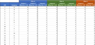
I have a group of companies in this table (see image and/or access link below), ranked based on 1 to 4, 1 being the lowest and 4 being the highest, on 8 different criteria in 3 different pillars. I intend to filter by values and find out the number of companies that meet at least one criteria in each pillar (which allows them to pass a certain assessment.

I had previously tried the FILTER function to get the number of companies that meet the 8 criteria individually and also in different combinations. But I am not sure how to go about filtering to find out the number of companies within a specific restriction in the criteria as underlined above.

Intended outcome: I hope to visualise (in a table or I am open to other suggestions) the number of companies, the criteria that they meet (which fall under the aim of having them meet at least one criteria in each pillar (which means that they would pass a certain assessment.

I have included the table in this link for easy access: Spreadsheet #2

Thank you!

 

[Eric W]

Welcome to the MrExcel forum!

I'm not sure what your preferred output is, but try:

Book1
	A	B	C	D	E	F	G	H	I	J	K	L	M
1			Pillar A			Pillar B			Pillar C
2	S/N	Company	Criteria 1 (Must be >2.2)	Criteria 2 (Must be >2.5)	Criteria 3 (Must be >3.3)	Criteria 4 (Must be >1.9)	Criteria 5 (Must be >2.3)	Criteria 6 (Must be >1.8)	Criteria 7 (Must be >2.9)	Criteria 8 (Must be >3.5)		Companies matching at least 1 criteria per pillar	Criteria passed
3	1	A	4	4	4	2	3	3	4	4		A	11111111
4	2	B	3	3	3	3	4	4	3	3		B	11011110
5	3	C	3	3	1	3	4	4	3	3		C	11011110
6	4	D	4	4	2	1	3	3	4	2		D	11001110
7	5	E	2	2	3	2	2	2	3	3		F	00111110
8	6	F	1	1	4	3	3	3	4	1		G	00110110
9	7	G	2	2	4	4	2	2	3	2		H	11010110
10	8	H	3	3	3	4	2	2	3	3		I	11111110
11	9	I	4	4	4	3	4	4	4	2		J	00110010
12	10	J	2	2	4	2	1	1	4	1		L	11111110
13	11	K	1	1	2	1	3	3	3	4		Q	11010110
14	12	L	3	3	4	4	3	3	3	3		R	11001111
15	13	M	2	2	2	3	2	2	3	3
16	14	N	1	1	3	3	4	4	2	2
17	15	O	2	2	4	1	3	3	1	1
18	16	P	4	4	2	1	4	4	1	2
19	17	Q	4	4	2	2	2	2	3	3
20	18	R	3	3	1	1	4	4	4	4
Sheet2

Cell Formulas
Range	Formula
L3:L14	L3	=FILTER(B3:B20,((C3:C20>2.2)+(D3:D20>2.5)+(E3:E20>3.3))*((F3:F20>1.9)+(G3:G20>2.3)+(H3:H20>1.8))*((I3:I20>2.9)+(J3:J20>3.5)))
M3:M20	M3	=IF(L3<>"",CONCAT((INDEX($C$3:$J$20,MATCH(L3,$B$3:$B$20,0),0)>{2.2,2.5,3.3,1.9,2.3,1.8,2.9,3.5})+0),"")
Dynamic array formulas.

 

[ShadowZeno]

Welcome to the MrExcel forum!

I'm not sure what your preferred output is, but try:

Book1
	A	B	C	D	E	F	G	H	I	J	K	L	M
1			Pillar A			Pillar B			Pillar C
2	S/N	Company	Criteria 1 (Must be >2.2)	Criteria 2 (Must be >2.5)	Criteria 3 (Must be >3.3)	Criteria 4 (Must be >1.9)	Criteria 5 (Must be >2.3)	Criteria 6 (Must be >1.8)	Criteria 7 (Must be >2.9)	Criteria 8 (Must be >3.5)		Companies matching at least 1 criteria per pillar	Criteria passed
3	1	A	4	4	4	2	3	3	4	4		A	11111111
4	2	B	3	3	3	3	4	4	3	3		B	11011110
5	3	C	3	3	1	3	4	4	3	3		C	11011110
6	4	D	4	4	2	1	3	3	4	2		D	11001110
7	5	E	2	2	3	2	2	2	3	3		F	00111110
8	6	F	1	1	4	3	3	3	4	1		G	00110110
9	7	G	2	2	4	4	2	2	3	2		H	11010110
10	8	H	3	3	3	4	2	2	3	3		I	11111110
11	9	I	4	4	4	3	4	4	4	2		J	00110010
12	10	J	2	2	4	2	1	1	4	1		L	11111110
13	11	K	1	1	2	1	3	3	3	4		Q	11010110
14	12	L	3	3	4	4	3	3	3	3		R	11001111
15	13	M	2	2	2	3	2	2	3	3
16	14	N	1	1	3	3	4	4	2	2
17	15	O	2	2	4	1	3	3	1	1
18	16	P	4	4	2	1	4	4	1	2
19	17	Q	4	4	2	2	2	2	3	3
20	18	R	3	3	1	1	4	4	4	4
Sheet2

Cell Formulas
Range	Formula
L3:L14	L3	=FILTER(B3:B20,((C3:C20>2.2)+(D3:D20>2.5)+(E3:E20>3.3))*((F3:F20>1.9)+(G3:G20>2.3)+(H3:H20>1.8))*((I3:I20>2.9)+(J3:J20>3.5)))
M3:M20	M3	=IF(L3<>"",CONCAT((INDEX($C$3:$J$20,MATCH(L3,$B$3:$B$20,0),0)>{2.2,2.5,3.3,1.9,2.3,1.8,2.9,3.5})+0),"")
Dynamic array formulas.

Hi! Could I know what does the second formula do? I understand the first part on the FILTER function but not the second one.

 

[Eric W]

Sure.

The MATCH part of the formula finds the row that corresponds to the value in column L. So if we're looking at company A, it returns C3::J3. Then it does a comparison of each of those values against the internal array, so C3>2.2, D3> 2.5, etc. That will return TRUE or FALSE for each comparison. If you add 0 to TRUE or FALSE, it becomes 1 or 0. Then finally the CONCAT concatenates the 1's and 0's together into an 8-digit string. So each digit represents one of your criteria, a 1 means it was met, a 0 means it wasn't. I didn't know how you wanted the results of the comparisons displayed, so I started with this. If you have a different idea, let me know.

Hope this helps!