ISNUMBER Find in text string with Date Range

Roxanne9876

New Member
Joined
Apr 6, 2022
Messages
5
Office Version
  1. 2021
Platform
  1. Windows
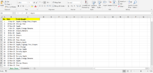
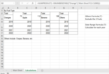
Hi. The main sheet contains information of the date and the fruits bought in each date. The second sheet (calculations sheet) contains the data I am calculating for.

Issues I faced:

1) I tried for many days to calculate the total number of fruits of each fruit type with date range as the criteria, however my formula is always wrong. I tried this: SUMPRODUCT(--('Main Sheet'!C2:C1000="Orange"),--('Main Sheet'!B2:B1000>="1/1/2019",<="12/31/2019"}) but it is an error.

2) For fruits other than the ones stated, I tried the formula: SUMPRODUCT(--ISNUMBER(FIND({"<>Banana","<>Apple","<>Oranges"},'Main Sheet'!C2:C1000))), however I still get an error.

Hopefully there will be a solution. Appreciate anyone for reading and helping.
 

Attachments

  • Image 1.png
    Image 1.png
    112.4 KB · Views: 19
  • Image 2.png
    Image 2.png
    42.7 KB · Views: 18
Tha
I would say a definite "No".

Using FIND with "Apple" would certainly cut out counting "Pineapple" but
- would miss out counting "apple" if it happened to be entered without the capital 'A'
- would still incorrectly count "Custard-Apple", "Rose-Apple" or "Sugar-Apple". It would also incorrectly count "Mangosteen" if using FIND with "Mango" etc.

What it is about my suggestion that ensures looking for correct words, & correct words only, is ensuring the word being looked for is enclosed between commas.

Also, the SUMPRODUCT suggestions above have a redundant year check
(YEAR('Main Sheet'!$B$2:$B$11)>=Calculations!A4)*(YEAR('Main Sheet'!$B$2:$B$11)<=Calculations!A4)
Since you are looking for a particular year with each formula, both the blue section and the red section do exactly the same job. For example, the only way a particular year can be >=2019 and <=2019 is if it is equal to 2019 so there is no need to check for it twice.

Another point about the previous SUMPRODUCT suggestions is that using the sheet name of the sheet that the formulas are actually on is a bad idea as it can lead to incorrect results.
=SUMPRODUCT((YEAR('Main Sheet'!$B$2:$B$11)>=Calculations!A4)*(YEAR('Main Sheet'!$B$2:$B$11)<=Calculations!A4)*ISNUMBER(FIND($C$3,'Main Sheet'!$C$2:$C$11)))
If you want to see what I mean, carefully follow through the steps of the example detailed in this post.

So, if you particularly want to use SUMPRODUCT (not a particularly efficient function) or need the solution to work in earlier versions of Excel then perhaps you could use this.

Roxanne9876.xlsm
BC
1DateFruits
23/09/2019Apple, Orange, Pear, Grapes
310/09/2019Orange, Pear, Custard-Apple
417/09/2019Apple
51/10/2020Apple, Orange, Banana
62/10/2020Grapes, Banana
73/10/2020Apple
815/10/2021Grapes
915/10/2021Pear
1015/10/2021Pear, Grapes
1115/10/2021Grapes, Apple
Main Sheet


Roxanne9876.xlsm
ABCDEFGH
3OrangeCountAppleCountBananaCountOthersCount
420192201922019020194
520201202022020220201
620210202112021020215
Calculations (4)
Cell Formulas
RangeFormula
B4:B6,F4:F6,D4:D6B4=SUMPRODUCT((YEAR('Main Sheet'!$B$2:$B$11)=A4)*ISNUMBER(SEARCH(", "&A$3&",",", "&'Main Sheet'!$C$2:$C$11&",")))
H4:H6H4=SUMPRODUCT((YEAR('Main Sheet'!B$2:B$11)=G4)*(LEN('Main Sheet'!C$2:C$11)-LEN(SUBSTITUTE('Main Sheet'!C$2:C$11,",",""))+1))-SUMIF(B$3:F$3,"Count",B4:F4)
Thank you for your detailed explanation. Appreciate that you took time out to help :)
 
Upvote 0

Excel Facts

How to calculate loan payments in Excel?
Use the PMT function: =PMT(5%/12,60,-25000) is for a $25,000 loan, 5% annual interest, 60 month loan.

Forum statistics

Threads
1,214,971
Messages
6,122,521
Members
449,088
Latest member
RandomExceller01

We've detected that you are using an adblocker.

We have a great community of people providing Excel help here, but the hosting costs are enormous. You can help keep this site running by allowing ads on MrExcel.com.
Allow Ads at MrExcel

Which adblocker are you using?

Disable AdBlock

Follow these easy steps to disable AdBlock

1)Click on the icon in the browser’s toolbar.
2)Click on the icon in the browser’s toolbar.
2)Click on the "Pause on this site" option.
Go back

Disable AdBlock Plus

Follow these easy steps to disable AdBlock Plus

1)Click on the icon in the browser’s toolbar.
2)Click on the toggle to disable it for "mrexcel.com".
Go back

Disable uBlock Origin

Follow these easy steps to disable uBlock Origin

1)Click on the icon in the browser’s toolbar.
2)Click on the "Power" button.
3)Click on the "Refresh" button.
Go back

Disable uBlock

Follow these easy steps to disable uBlock

1)Click on the icon in the browser’s toolbar.
2)Click on the "Power" button.
3)Click on the "Refresh" button.
Go back
Back
Top