Iterative Calculations and Match issues with out of range values.

[RainGauge]

I've hit a wall and am not certain how to proceed. Any help is appreciated!

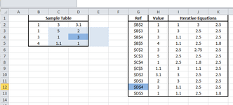
The attached image is a representation of my worksheet which is much larger.

Problem: Column I & J & K is to be populated with an equation that iteratively calculates the median of its neighboring cells. Column I uses H, while J uses I and K uses J.

Column G and H are paired datasets that represent information pulled from a table, G being the cell reference and H being its value.

The goal of the equation is to have it take the cell reference in column G and then find the neighboring cells of its INDIRECT reference, ex: D4 would calculate the median of C3,C4,C5,D3,D5 (and E3,E4,E5 assuming they weren't off the table).

This is what I've come up with:
=MEDIAN(INDEX(H$2:H$13,TARGET CELL,TARGET CELL2,TARGET CELL3,TARGET CELL4,TARGET CELL5,TARGET CELL6,TARGET CELL7,TARGET CELL8)

Each TARGET CELL has a variation of the following, where the offset is modified to target a different direction:
MATCH(ADDRESS(ROW(OFFSET(INDIRECT($G2),0,-1)),COLUMN(OFFSET(INDIRECT($G2),-1,0))),$G$2:$G$13,0))

It gives me an #N/A error when MATCH attempts to return a value that has no match in column G (It's value is at the edge of the table).
Is there a way to have my equation calculate the median while discarding the match results that return #N/A?

I was hoping to have this all calculated in single cells, but if it isn't possible I am aware that I can calculate each neighboring cell in its own helper column then discard the errors.
Is there a better approach or a solution that doesn't involve 8 helper columns? Thanks in advance for taking the time to read my question.

 

[StephenCrump]

Welcome to the Forum!

I think this what you're describing, but I don't follow what you're doing in the iterations:

	A	B	C	D	E	F	G	H	I	J	K
1		Sample						Sample
2
3		2.0	3.0	3.1				2.0	3.0	3.1
4		1.0	5.0	2.0				1.0	5.0	2.0
5		3.0	1.0	3.0				3.0	1.0	3.0
6		4.0	1.1	1.0				4.0	1.1	1.0
7
8		Median						Median
9		3.0	2.0	3.0				3.0	2.0	3.0
10		3.0	2.5	3.0				3.0	2.5	3.0
11		1.1	2.5	1.6				1.1	2.5	1.1
12		1.1	3.0	1.1				1.1	3.0	1.1
13
14		3.0							1.0
15		1.0							5.0
16		5.0							2.0
17		3.0							3.0
18									3.0
19									4.0
20									1.1
21									1.0
22									2.5
23
Sheet1

Cell Formulas
Range	Formula
B9:C9,H9:I9	B9	=MEDIAN(A1:C1,A4:C4,A3,C3)
D9,J9	D9	=MEDIAN(C1:J1,C4:J4,C3,J3)
B10:C11,H10:I11	B10	=MEDIAN(A3:C3,A5:C5,A4,C4)
D10:D11,J10:J11	D10	=MEDIAN(C3:J3,C5:J5,C4,J4)
B12:C12,H12:I12	B12	=MEDIAN(A5:C5,A8:C8,A6,C6)
D12,J12	D12	=MEDIAN(C5:J5,C8:J8,C6,J6)
B14	B14	=C3
B15,I15	B15	=B4
B16,I16	B16	=C4
B17	B17	=MEDIAN(B14:B16)
I14	I14	=H4
I17	I17	=H5
I18	I18	=J5
I19	I19	=H6
I20	I20	=I6
I21	I21	=J6
I22	I22	=MEDIAN(I14:I21)

 

[RainGauge]

Thanks for the response.

I realize I could have been more clear about what was the purpose of the equation and what I was trying to achieve. In case you're curious, I was working with a large dataset of weather radar data that contained obviously erroneous data. The goal of the exercise was to approximate the value of cells that contained these errors using its surrounding data. The multiple passes (the iteration) was to stabilize the data in case an erroneous cell was adjacent to another erroneous cell.

I ended up creating multiple iterations of the entire table each referring to its previous incarnation. Regardless, I found a solution and the problem is solved.