Large Data Sets Into Schedules

[davidmel20]

Hi, I tried a lot of things for this but unfortunately I'm not well-versed enough in VBA to get what I need done and couldn't find any other related posts, so I'm coming to the experts!

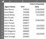
I have a data set that includes 20 or so columns but I only need to reference three fields, "Agent", "ID #" and "Ticket Scheduled Date" (In the normal report, these will not be in columns A, B and C as they are in the example). There are a few things that I'm trying to make happen...

I've attached a few images of the data and what the end result would look like.
1) Based on the values that I put in sheet "Schedule", cells D1 and G1, create dates going across beginning in C5 until the date that's populated in G1.
2) Populate column B ("Agent Name") and the corresponding ID number relative to the scheduled date across the top. The data for this is in sheet "Data". If there is someone in the "Data" sheet that doesn't have a ticket scheduled within the dates that I've populated, I don't want them to show up. Some agents may have multiple ticket ID's for one day also.
3) Based on the value of the ID #, the color coding needs to change (over 600000 vs under 600000). I'm aware this can be done with conditional formatting but I'm not sure if it would be easier to just include in a macro.

I'm looking to make this as simple as possible, probably via a button or msg box, as it will be for entry-level employees to update the "Data" tab and then run the updates. Any help is greatly appreciated and thank you in advance.

 

[Peter_SSs]

Welcome to the MrExcel board!

For the future, I would strongly recommend providing any sample data using XL2BB as helpers are reluctant to spend a lot of time manually typing out sample data to test with.

Anyway, give this a try in a copy of your workbook to see if it is close to the mark.

Sub MakeSchedule()
  Dim a As Variant
  Dim StartDate As Date, Enddate As Date
  Dim NumDays As Long, c As Long, r As Long, i As Long
  
  a = Sheets("Data").Range("A2", Sheets("Data").Range("C" & Rows.Count).End(xlUp)).Value
  With Sheets("Schedule")
    .UsedRange.Offset(4).Clear
    StartDate = .Range("D1").Value
    Enddate = .Range("G1").Value
    NumDays = Enddate - StartDate + 1
    .Cells(5, 2).Value = "Agent Name"
    For c = 0 To NumDays - 1
      .Cells(5, 3 + c).Value = StartDate + c
    Next c
    r = 5
    For i = 1 To UBound(a)
      If a(i, 3) >= StartDate And a(i, 3) <= Enddate Then
        c = a(i, 3) - StartDate
        r = r + 1
        .Cells(r, 2).Value = a(i, 1)
        With .Cells(r, 3 + c)
          .Value = a(i, 2)
          .Interior.ColorIndex = IIf(a(i, 2) > 600000, 40, 50)
        End With
      End If
    Next i
  End With
End Sub

 

[davidmel20]

This is PERFECT! I updated the code below to make a few minor changes, adding a few columns with more data (customer, location, revenue and status). Is there any chance we can add these in? I tried to add these fields in myself to pull from the ticket ID but am having trouble with filling down the correct number of rows, I basically just added in a vlookup which probably isn't the ideal way to go. I've also put in the XL2BB . These are the final changes that I'm hoping to add in:
-Add "Customer", "Location", "Revenue $" and "Status" from Data sheet based off of the ticket ID
-Format the column width to 11 only for the added dates across row 5 (F5:5)
-For all values in row 5, format the font the same way (blue fill & bold)

Sub MakeSchedule()
  Dim a As Variant
  Dim StartDate As Date, Enddate As Date
  Dim NumDays As Long, c As Long, r As Long, i As Long
  
  a = Sheets("Data").Range("A2", Sheets("Data").Range("C" & Rows.Count).End(xlUp)).Value
  With Sheets("Schedule")
    .UsedRange.Offset(4).Clear
    StartDate = .Range("C1").Value
    Enddate = .Range("F1").Value
    NumDays = Enddate - StartDate + 1
    .Cells(5, 1).Value = "Agent Name"
    .Cells(5, 2).Value = "Customer"
    .Cells(5, 3).Value = "Location"
    .Cells(5, 4).Value = "Revenue $"
    .Cells(5, 5).Value = "Status"
    For c = 0 To NumDays - 1
      .Cells(5, 6 + c).Value = StartDate + c
    Next c
    r = 5
    For i = 1 To UBound(a)
      If a(i, 3) >= StartDate And a(i, 3) <= Enddate Then
        c = a(i, 3) - StartDate
        r = r + 1
        .Cells(r, 1).Value = a(i, 1)
        With .Cells(r, 6 + c)
          .Value = a(i, 2)
          .Interior.ColorIndex = 40
        End With
      End If
    Next i
  End With
End Sub

mrexelmacro_w customer.xlsm
	A	B	C	D	E	F	G
1	Agent Name	ID #	Ticket Scheduled Date	Customer	Location	Revenue $	Status
2	Max Brown	479156	2/28/2020	Customer A	SITE 123	$ 3,000.00	Schedule Due
3	Janet Black	437218	2/29/2020	Customer B	SITE 356	$ 5,000.00	Assigned
4	David White	333493	3/1/2020	Customer C	SITE 722	$ 8,000.00	In Process
5	Bob Purple	486878		Customer D	SITE 843	$ 2,000.00	Schedule Due
6	Karen Blue	452388	2/28/2020	Customer E	SITE 223	$ 4,500.00	Assigned
7	John Purple	584910		Customer F	SITE 128	$ 8,700.00	In Process
8	Adrian Aqua	430105	3/4/2020	Customer G	SITE 169	$ 9,300.00	Schedule Due
9	Adrian Aqua	946331	3/4/2020	Customer H	SITE 453	$ 1,600.00	Assigned
10	Phil Magenta	284020		Customer I	SITE 954	$ 8,300.00	In Process
11	Carrie Green	187810	3/6/2020	Customer J	SITE 100	$ 5,600.00	Assigned
Data

mrexelmacro_w customer.xlsm
	A	B	C	D	E	F	G	H	I	J	K	L
1	Schedule Start Date:		2/27/2020	Schedule End Date:		3/4/2020
2
3
4						TICKET SCHEDULED DATE
5	Agent Name	Customer	Location	Revenue $	Status	2/27/2020	2/28/2020	2/29/2020	3/1/2020	3/2/2020	3/3/2020	3/4/2020
6	Max Brown						479156
7	Janet Black							437218
8	David White								333493
9	Karen Blue						452388
10	Adrian Aqua											430105
11	Adrian Aqua											946331
Schedule

 

[Peter_SSs]

Thanks for using XL2BB - makes things much easier.

Give this version a try.
Notes:

1. The code does not alter the column widths so set them manually how you want (eg columns F:?? to width 11) & they should remain unchanged.
2. You didn't mention changing the two-tone colour arrangement though I notice your code has reverted to a single colour. I have left the 2-colour arrangement in place (though implemented a little differently).

Sub MakeSchedule_v2()
  Dim a As Variant
  Dim StartDate As Date, Enddate As Date
  Dim NumDays As Long, c As Long, r As Long, i As Long
 
  a = Sheets("Data").Range("A2", Sheets("Data").Range("G" & Rows.Count).End(xlUp)).Value
  With Sheets("Schedule")
    .UsedRange.Offset(5).Clear
    .UsedRange.Offset(4, 6).Clear
    StartDate = .Range("C1").Value
    Enddate = .Range("F1").Value
    NumDays = Enddate - StartDate + 1
    With .Range("F5").Resize(, NumDays)
      .Cells(1).Copy Destination:=.Cells(1).Resize(, NumDays)
      .Value = Application.Transpose(Evaluate("Row(" & CLng(StartDate) & ":" & CLng(StartDate) + NumDays - 1 & ")"))
    End With
    r = 5
    For i = 1 To UBound(a)
      If a(i, 3) >= StartDate And a(i, 3) <= Enddate Then
        r = r + 1
        .Cells(r, 1).Resize(, 5).Value = Application.Index(a, i, Array(1, 4, 5, 6, 7))
        c = a(i, 3) - StartDate
        With .Cells(r, 6 + c)
          .Value = a(i, 2)
          .Interior.Color = IIf(a(i, 2) > 600000, RGB(255, 204, 153), RGB(196, 215, 155))
        End With
      End If
    Next i
  End With
End Sub

 

[davidmel20]

Exactly what I need, thank you so much peter!

 

[Peter_SSs]

Exactly what I need, thank you so much peter!

Glad to help. Thanks for the follow-up.