Line of worst fit !

Getafix1066

Board Regular
Joined
May 15, 2016
Messages
57
Line of best fit that isn’t.

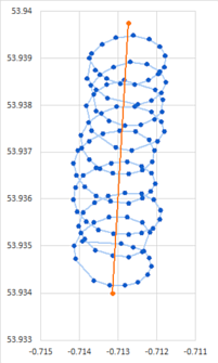
Have a look at this graph. It shows the latitude and longitude of a paraglider circling whilst drifting over the ground….
185x135.png


(if I’ve clicked the correct buttons, a good quality image of the graph called ‘LineOfworstFit.png’ should be here http://ge.tt/1cadawo2 )

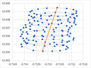
The image clearly shows that a line-of-best-fit (aka a trend line) should be almost vertical (north-south), but the trend line added by excel is at a 45 degree angle (as shown)

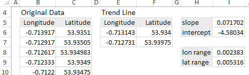
After much head scratching I figured out why – it’s because the scales on the each axis aren’t equal, basically one unit of latitude on the vertical scale (Y) represents a different distance to one unit of longitude on the horizontal scale (X)

My question is - how to create a line-of-best-fit that matches the drift of the aircraft? The graph itself isn't complex, and the trend line function is performing correctly, but the result doesn't match the 'common sense' result expected.

(a simple spreadsheet containing the data and the graph is available at the above link)

Thanks
 

Excel Facts

Who is Mr Spreadsheet?
Author John Walkenbach was Mr Spreadsheet until his retirement in June 2019.
I think this is what you want.

You want to calculate your own trend line and add it as a second series. The x values will be the latitude and the y values will be the longitude.

H2cKNaQ.png


In I5: =SLOPE(B6:B128, C6:C128)
In I6: =INTERCEPT(B6:B128, C6:C128)

F6 and F7 are manually entered; the latitude points were chosen to lie just above and below the collected values.

In E6: =$I$5*F6+$I$6
In E7: =$I$5*F7+$I$6

Chart the original data as a scatter plot.
Copy E5:F7.
Select the chart.
From the Home tab, select the dropdown menu below the large Paste icon then select "Paste Special...".
The selections on the popup menu should be:

3dkEuK7.png


Format as you would wish:

a6v98eb.png


My workbook: https://www.dropbox.com/s/pyx1tdyvnaohlgm/aircraft_drift.xlsx?dl=0
 
Upvote 0
Thanks thisoldman,

The line you've plotted is exactly what I wanted - except that I need to do it automatically! The method proposed relies on the manual selection of the two points at the end of the orange line (unless I've mis-understood).

I've done some more reading since my original post. The excel trend-line relies on something called the least-squares method, which (apparently) won't provide good fits for vertical data points. What I'm still trying to find out is how to do what you've shown automatically.

Thank you
 
Upvote 0
If you switch latitude and longitude axes, the Excel chart trendline will work as you want. But you will create confusion for the viewer as latitude and longitude are not as they would appear on a map. See the second tab in my uploaded workbook. The slope and intercept functions do use a least-squares method, the same as clicking the option for a chart.

To automate the chart, use a scatterplot with two series. Where I manually selected the two points for the end points of the trend line, use the max and min of the latitude.

F6: =MIN(C6:C128)
F7: =MAX(C6:C128)

See the new third tab in my uploaded workbook.
If you want to do this automatically for a varying count of positional data, say up to 500 points, we can use a dynamic range to calculate the minimum and maximum latitudes.

F6: =MIN(C6:INDEX(C6:C506, COUNT(C6:C506)))
F7: =MAx(C6:INDEX(C6:C506, COUNT(C6:C506)))

I show this dynamic range formula on the third tab of the worksheet also.
 
Last edited:
Upvote 0
Thanks thisoldman,

I've re-read your post, and (if I understand correctly) excel will return different values of SLOPE() and INTERCEPT() depending on which axis is treated as 'x' and which as 'y' - so switching the two axis around you get a better fit.

But there still remains the question of how to do this automatically? - if the wind is blowing from east to west then the fixes will be spread from left to right, and the first method for finding the trend line is probably best, but in other cases (north/south) then the 2nd method is better
 
Upvote 0
If you are OK with a separate series for the trend line, we can automate which trend line is displayed using formulas.

I do use named formulas to create dynamic ranges for the collected latitude and longitude data.


Book1
BCDEF
4Original DataTrend Line
5LongitudeLatitudeLongitudeLatitude
6-0.71391753.9351-0.71313153.934167
7-0.71291753.93505-0.7127553.939483
8-0.71261753.934983
9-0.71233353.9349
Sheet1
Cell Formulas
RangeFormula
E6=IF(ABS(MAX(Latitude) - MIN(Latitude)) > ABS(MAX(Longitude) - MIN(Longitude)), SLOPE(Longitude, Latitude) * MIN(Latitude) + INTERCEPT(Longitude, Latitude), MIN(Longitude))
E7=IF(ABS(MAX(Latitude) - MIN(Latitude)) > ABS(MAX(Longitude) - MIN(Longitude)), SLOPE(Longitude, Latitude) * MAX(Latitude) + INTERCEPT(Longitude, Latitude), MAX(Longitude))
F6=IF(ABS(MAX(Latitude) - MIN(Latitude)) < ABS(MAX(Longitude) - MIN(Longitude)), SLOPE(Latitude, Longitude) * MIN(Longitude) + INTERCEPT(Latitude, Longitude), MIN(Latitude))
F7=IF(ABS(MAX(Latitude) - MIN(Latitude)) < ABS(MAX(Longitude) - MIN(Longitude)), SLOPE(Latitude, Longitude) * MAX(Longitude) + INTERCEPT(Latitude, Longitude), MAX(Latitude))
Named Ranges
NameRefers ToCells
Latitude=Sheet1!$C$6:INDEX(Sheet1!$C$6:Sheet1!$C$506,COUNT(Sheet1!$C$6:Sheet1!$C$506))
Longitude=Sheet1!$B$6:INDEX(Sheet1!$B$6:Sheet1!$B$506,COUNT(Sheet1!$B$6:Sheet1!$B$506))

New workbook: https://www.dropbox.com/s/fshon0pmbpd7xfi/aircraft_drift_v2.xlsx?dl=0
 
Last edited:
Upvote 0
Thank you for your help thisoldman.

What I've learnt elsewhere is that the SLOPE() and INTERCEPT() functions use 'least squares' regression which depends on which set of data you specify as the X and Y axis.

Apparently there's something called 'total least squares' regression which is independent of which is the 'x' and 'y' axis, unfortunately there doesn't seem to be a simple excel function to give this.
 
Upvote 0
Well, that's good. I felt the linear regression would not accurately show the drift. I avoided showing my misgivings because I assumed a proper solution would require a bunch of trigonometry and array formulas. It turns out, we can use Excel statistical functions to determine the total least squares.

I used the method shown by Charles Zaiontz at "Real Statistics Using Excel", http://www.real-statistics.com/regression/total-least-squares/.

Again I used named formulas for Latitude and Longitude. I also used a bunch of named cells—I needed to follow the formula logic and named formulas make that much easier than using Excel references. To reduce complexity, I did not combine formulas, even though the opportunities to do so may seem obvious.

The solution I came up with is similar to my last post—the trend line is a second series. To make the trend line display stay within the limits of the observed data, so that reasonable axes limits are maintained, I created a trend line takes into account the relative sizes of the latitude and longitude ranges. This means if the longitude range is greater than the latitude range, I use longitude as the independent variable, the x value in the line formula y = mx + b. If the latitude range is greater, latitude is used as the x in y = mx + b.


Book1
BCDEFGHI
7Original DataTrend LineCalculations
8LongitudeLatitudeLonLatMinimum Longitude-0.71415
9-0.7139253.9351-0.7132453.93417Maximum Longitude-0.711767
10-0.7129253.93505-0.712653.93948Longitude Range0.002383
11-0.7126253.93498Minimum Latitude53.934167
12-0.7123353.9349Maximum Latitude53.939483
13-0.712253.93475Latitude Range0.005316
14-0.7121553.93457Mean Longitude-0.71292197
15-0.7122353.9344Mean Latitude53.93682446
16-0.7124853.93423Observations120
17-0.7128253.93417Independent VariableLatitude
18-0.7132253.93417W_-0.00017971
19-0.7136253.93427R_4.38389E-05
20-0.714153.93473Slope0.120211916
21-0.7141353.935Intercept-7.19677099
Sheet1
Cell Formulas
RangeFormula
E9=IF(IndepVar = "Longitude", MinLongitude, TrendSlope * MinLatitude + TrendIntercept)
E10=IF(IndepVar = "Longitude", MaxLongitude, TrendSlope * MaxLatitude + TrendIntercept)
F9=IF(IndepVar = "Longitude", TrendSlope * MinLongitude + TrendIntercept, MinLatitude)
F10=IF(IndepVar = "Longitude", TrendSlope * MaxLongitude + TrendIntercept, MaxLatitude)
I8=MIN(Longitude)
I9=MAX(Longitude)
I10=ABS(MaxLongitude - MinLongitude)
I11=MIN(Latitude)
I12=MAX(Latitude)
I13=ABS(MaxLatitude - MinLatitude)
I14=AVERAGE(Longitude)
I15=AVERAGE(Latitude)
I16=COUNT(Longitude)
I17=REPT("Longitude", LonRange > LatRange) & REPT("Latitude", LonRange <= LatRange)
I18=IF(IndepVar = "Longitude", DEVSQ(Latitude) - DEVSQ(Longitude), DEVSQ(Longitude) - DEVSQ(Latitude))
I19=2 * COVARIANCE.P(Longitude, Latitude) * Observations
I20=(W_ + SQRT(W_^2 + R_^2)) / R_
I21=IF(IndepVar = "Longitude", MeanLat - MeanLon * TrendSlope, MeanLon - MeanLat * TrendSlope)
Named Ranges
NameRefers ToCells
IndepVar=Sheet1!$I$17
Latitude=Sheet1!$C$6:INDEX(Sheet1!$C$6:Sheet1!$C$506,COUNT(Sheet1!$C$6:Sheet1!$C$506))
LatRange=Sheet1!$I$13
Longitude=Sheet1!$B$6:INDEX(Sheet1!$B$6:Sheet1!$B$506,COUNT(Sheet1!$B$6:Sheet1!$B$506))
LonRange=Sheet1!$I$10
MaxLatitude=Sheet1!$I$12
MaxLongitude=Sheet1!$I$9
MeanLat=Sheet1!$I$15
MeanLon=Sheet1!$I$14
MinLatitude=Sheet1!$I$11
MinLongitude=Sheet1!$I$8
Observations=Sheet1!$I$16
R_=Sheet1!$I$19
TrendIntercept=Sheet1!$I$21
TrendSlope=Sheet1!$I$20
W_=Sheet1!$I$18

ZRfq72m.png


New workbook at: https://www.dropbox.com/s/bdnluvqptvi612r/aircraft_drift_v3.xlsx?dl=0
 
Upvote 0
Thanks @thisoldman - following some of your earlier tips I to had come across real-statistics.com and had been adapting it to use 'total least squares'. I had hoped (as per my other recent post on this forum) that the total least squares technique would be a standard excel feature, but apparently not! Thanks again.
 
Upvote 0

Forum statistics

Threads
1,214,622
Messages
6,120,580
Members
448,972
Latest member
Shantanu2024

We've detected that you are using an adblocker.

We have a great community of people providing Excel help here, but the hosting costs are enormous. You can help keep this site running by allowing ads on MrExcel.com.
Allow Ads at MrExcel

Which adblocker are you using?

Disable AdBlock

Follow these easy steps to disable AdBlock

1)Click on the icon in the browser’s toolbar.
2)Click on the icon in the browser’s toolbar.
2)Click on the "Pause on this site" option.
Go back

Disable AdBlock Plus

Follow these easy steps to disable AdBlock Plus

1)Click on the icon in the browser’s toolbar.
2)Click on the toggle to disable it for "mrexcel.com".
Go back

Disable uBlock Origin

Follow these easy steps to disable uBlock Origin

1)Click on the icon in the browser’s toolbar.
2)Click on the "Power" button.
3)Click on the "Refresh" button.
Go back

Disable uBlock

Follow these easy steps to disable uBlock

1)Click on the icon in the browser’s toolbar.
2)Click on the "Power" button.
3)Click on the "Refresh" button.
Go back
Back
Top