List of Tab Names

[butch3]

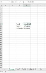
When excel starts, I'd like the list of tab names (after the first tab) to populate as a list in the first tab starting from G9 and going down. In H9, going down, the macro should just simply display what is in each tab on cell B4 (except for the first tab).

It is preferred that only the G9, H9, and the data being displayed as a result of this program be placed in order of the earliest date. G5, for example, should not be sorted since this is outside of the area for this program.

Tabs may be added or modified in the future by the user. Also, there may be other text on the sheet for the first tab. This code should not interfere with the text that is in other columns.

 

[BSALV]

Sub List_TabNames()

     Dim arr()                                                  'tempory array to stock data
     ReDim arr(1 To 2, 1 To 10)                                 'already made for 10 worksheets

     For i = 2 To ThisWorkbook.Worksheets.Count                 'loop through all worksheets
          ptr = ptr + 1                                         'pointer
          If ptr > UBound(arr, 2) Then ReDim Preserve arr(1 To 2, 1 To ptr)     'if array isn't great enough redim & keep actual datat
          With Worksheets(i)
               arr(1, ptr) = .Name                              'the name of that worksheet
               arr(2, ptr) = .Range("B4").Value2                'the value of B4
          End With
     Next

     With Sheets(1).Range("G9")                                 'on the 1st worksheet
          .Resize(100, 2).ClearContents                         'clear contents of 100*2 cells starting in G9
          With .Resize(UBound(arr, 2), UBound(arr))             'this is the size of the range to be written
               .Value = Application.Transpose(arr)              'write the transposed array
               .Sort .Range("B1"), xlAscending, Header:=xlNo    'sort on the 2nd column
          End With
     End With

End Sub

 

[Eric W]

Consider:

First go to the name manager and create a named range called SheetNames with this formula:

=TRANSPOSE(GET.WORKBOOK(1)&T(NOW()))

Then create a sheet as below:

Book1
	A	B	C	D	E	F	G	H
1
2
3
4
5
6
7
8
9				Sheet33			Sheet24	10/1/2021
10				Sheet34			Sheet3	12/25/2021
11				Sheet24	10/1/2021		Sheet33
12				Sheet3	12/25/2021		Sheet34
13				Sheet35	1/3/2022		Sheet35	1/3/2022
14				Sandbox	2/2/2022		Sandbox	2/2/2022
15
Sheet34

Cell Formulas
Range	Formula
D9:E14	D9	=SORT(CHOOSE({1,2},MID(SheetNames,FIND("]",SheetNames)+1,255),SUMIF(INDIRECT("'"&MID(SheetNames,FIND("]",SheetNames)+1,255)&"'!B4"),">0")),2)
G9:G15	G9	=IFERROR(INDEX(MID(SheetNames,FIND("]",SheetNames)+1,255),ROWS(G$9:G9)),"")
H9:H15	H9	=IF(G9="","",SUMIF(INDIRECT("'"&G9&"'!B4"),">0"))
Dynamic array formulas.

If you don't have Excel 365, use the G9:H9 formulas and drag down. If you have Excel 365, the D9 formula will work, and it sorts the sheets by date. I used a custom number format of

m/d/yyyy;;;

so that non-date entries would not show up. For either version, you'll need to save the workbook as macro-enabled.

 

[butch3]

Sub List_TabNames()

     Dim arr()                                                  'tempory array to stock data
     ReDim arr(1 To 2, 1 To 10)                                 'already made for 10 worksheets

     For i = 2 To ThisWorkbook.Worksheets.Count                 'loop through all worksheets
          ptr = ptr + 1                                         'pointer
          If ptr > UBound(arr, 2) Then ReDim Preserve arr(1 To 2, 1 To ptr)     'if array isn't great enough redim & keep actual datat
          With Worksheets(i)
               arr(1, ptr) = .Name                              'the name of that worksheet
               arr(2, ptr) = .Range("B4").Value2                'the value of B4
          End With
     Next

     With Sheets(1).Range("G9")                                 'on the 1st worksheet
          .Resize(100, 2).ClearContents                         'clear contents of 100*2 cells starting in G9
          With .Resize(UBound(arr, 2), UBound(arr))             'this is the size of the range to be written
               .Value = Application.Transpose(arr)              'write the transposed array
               .Sort .Range("B1"), xlAscending, Header:=xlNo    'sort on the 2nd column
          End With
     End With

End Sub

Code seems good. The only issue is that the output includes hidden tabs. I don't want hidden tabs to be listed. Thanks.

 

[Fluff]

What version of Excel are you using?

I suggest that you update your Account details (or click your user name at the top right of the forum) so helpers always know what Excel version(s) & platform(s) you are using as the best solution often varies by version. (Don’t forget to scroll down & ‘Save’)

Another option, depending on version

Sub butch()
   Dim Ary As Variant
   Dim Ws As Worksheets
   Dim i As Long
   
   ReDim Ary(1 To Worksheets.Count - 1, 1 To 2)
   For i = 2 To Worksheets.Count
      With Worksheets(i)
         Ary(i - 1, 1) = .Name
         Ary(i - 1, 2) = .Range("B4").Value
      End With
   Next i
   Sheets(1).Range("G9").Resize(UBound(Ary), 2).Value = Application.Sort(Ary, 2)
End Sub

 

[BSALV]

Sub butch()
     Dim Ary   As Variant
     Dim Ws    As Worksheets
     Dim i     As Long

     ReDim Ary(1 To Worksheets.Count - 1, 1 To 2)
     For i = 2 To Worksheets.Count
          With Worksheets(i)
               If .Visible Then
                    ptr = ptr + 1
                    Ary(ptr, 1) = .Name
                    Ary(ptr, 2) = .Range("B4").Value
               End If
          End With
     Next i
     Sheets(1).Range("G9").Resize(UBound(Ary), 3).Value = Application.Sort(Ary, 2)
End Sub