listbox selection

[ttowncorp]

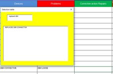
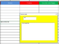
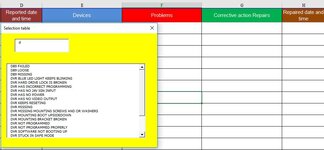
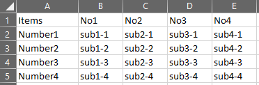
I have a list box with a dropdown list i created for testing and I want to see how can I select a specific word from my drop down list in one cell, and in the next cell depending on my previous selection only shows what that selection is tied to. so for example. E1 I select "DB9 connector". When i go to F1 and go to my dropdown list it will only show all my different DB9 connector problems only and not my other DB9 problems. My list under FI will have hundreds of different type of problem scenario for me to choose from so I want to make it easier by not having to scroll through so many in my dropdown list. how would a code like that look like? And make it a way so people can not free type in these cells but can only choose from what they select. I been wanting to do this for years but could never really get any help on coding.

 

[Candyman8019]

Use Named Ranges for this exercise.
On a separate sheet (refer to attached pic), column 1 will be your first dropdown menu. specify the column as named range "items"...Then set your data validation cell to return your list of "items".
Column B...call this range "Number1"
Column C...call this range "Number2"...etc.

In your second validation field specify the list with the following formula: =INDIRECT({cell of first validation field})
This will match your selection in the first validation field with the named range that lists a sub-selection of values.

 

[ttowncorp]

Use Named Ranges for this exercise.
On a separate sheet (refer to attached pic), column 1 will be your first dropdown menu. specify the column as named range "items"...Then set your data validation cell to return your list of "items".
Column B...call this range "Number1"
Column C...call this range "Number2"...etc.

In your second validation field specify the list with the following formula: =INDIRECT({cell of first validation field})
This will match your selection in the first validation field with the named range that lists a sub-selection of values.

okay i was trying to get this to work out, and i'm not to good in coding much, but i'm i using the formula as =indirect(a2-a5)

 

[Candyman8019]

If your first validation field is in Cell A1 and your second validation field is in B1, then the validation formula for B1 would be =INDIRECT(A1)

 

[ttowncorp]

If your first validation field is in Cell A1 and your second validation field is in B1, then the validation formula for B1 would be =INDIRECT(A1)

thanks for the help but i guess i just have no clue as to making this still work the way i like to.

 

[Candyman8019]

Looking back at your original post, you mention that you have a list of hundreds of problem scenarios. You will need to break those down into multiple lists that correspond with the values you have populated in E1.

Book2
	A	B	C	D	E	F	G	H
1	connectors	DB9 Connector	HDMI Connector	RJ45 Connector			DB9_connector
2	DB9_connector	problem 1	problem 1	problem 1
3	HDMI_Connector	problem 2	problem 2	problem 2
4	RJ45_Connector	problem 3	problem 3	problem 3
5		problem 4	problem 4
6		problem 5	problem 5
7		problem 6	problem 6
8			problem 7
9			problem 8
10			problem 9
11			problem 10
12
Sheet1

Cells with Data Validation
Cell	Allow	Criteria
G4	List	1,23,3
G1	List	=Connectors
H1	List	=INDIRECT(G1)

 

[Candyman8019]

In the above example, I used named ranges, for example, range B2:B7 was named "DB9_Connector"...the same as an option in my first dropdown field. C2:C11 is named "HDMI_Connector", etc.

 

[ttowncorp]

Looking back at your original post, you mention that you have a list of hundreds of problem scenarios. You will need to break those down into multiple lists that correspond with the values you have populated in E1.

Book2
	A	B	C	D	E	F	G	H
1	connectors	DB9 Connector	HDMI Connector	RJ45 Connector			DB9_connector
2	DB9_connector	problem 1	problem 1	problem 1
3	HDMI_Connector	problem 2	problem 2	problem 2
4	RJ45_Connector	problem 3	problem 3	problem 3
5		problem 4	problem 4
6		problem 5	problem 5
7		problem 6	problem 6
8			problem 7
9			problem 8
10			problem 9
11			problem 10
12
Sheet1

Cells with Data Validation
Cell	Allow	Criteria
G4	List	1,23,3
G1	List	=Connectors
H1	List	=INDIRECT(G1)

oh wow, now I see it. this makes more since now seeing your example this way. thank you for being patient.