Locking a number from resetting to zero

[SpikeL]

Good afternoon. first post.
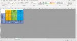
I am by no means an expert but i can do the basics in Excel (2016). i have created a simple data capture sheet that is used weekly in a briefing (copied and pasted to PowerPoint). On the left i have a list of activities (A5-A11). Columns B5-11 and C5-11 represent the previous month (i input numbers for two separate activities) Columns D,E, represent the current with F,G representing the future.B-G 12 represent a total of each of the above while B13 and 14 would be a 'rolling' total of D,E 13 respectively (with the raw data being taken from D,E as my current month).
I hope that kind of makes sense? what i am trying to achieve is that B13 and 14 remain the accumulative (rolling) totals so when i remove the numbers from D&E 5-11, it doesn't affect the total (but only if i have to adjust a number say from 5 to 4)

ill see if i can upload an image.

 

[J.Ty.]

Hi,

Welcome to the Board!

1) The spreadsheet software has no method to understand by itself the difference between adjusting a few numbers in D5:E11, and adjusting all of them one by one, to get the values for the next period.
2) Therefore there must be a special method to tell the spreadsheet "I am doing adjustments now" and "I am moving to the next period now", and the reactions to changes in each case should be different.
3) That being said, I can do this using formulas and circular references. It will work, but I do not recommend it, because it is a fragile mechanism, relatively sensitive to human errors. Therefore I think VBA is the technology to use, but this is not my area.

J.Ty.

 

[SpikeL]

Hi,

Welcome to the Board!

1) The spreadsheet software has no method to understand by itself the difference between adjusting a few numbers in D5:E11, and adjusting all of them one by one, to get the values for the next period.
2) Therefore there must be a special method to tell the spreadsheet "I am doing adjustments now" and "I am moving to the next period now", and the reactions to changes in each case should be different.
3) That being said, I can do this using formulas and circular references. It will work, but I do not recommend it, because it is a fragile mechanism, relatively sensitive to human errors. Therefore I think VBA is the technology to use, but this is not my area.

J.Ty.

Thanks for the reply. As I have limited knowledge on VBA I may have to accept defeat. I may just have to input that bit manually but just keep a record on another sheet just in case

 

[J.Ty.]

You can have a look at my solution, being aware of its defects.
It requires the following steps:

1) Go to File->Options->Formulas->Enable iterative calculation and check it, set "Maximum iterations" to 1.
2) Copy formulas
3) As long as B14 is "LOCKED" you can change the values in the orange area and the sum in the blue cell is the sum of them and B15.
4) When you change B14 to "UPDATE", the sum is transferred and added to B15.
5) When you then change B14 to "LOCKED" again, the orange area becomes separated from B15 and you can put the date for a new period there and adjust them.
6) For security, there is a data validation in B14, which allows only "LOCKED" and "UPDATE" there, but it i not necessary for making experiments.
7) However, if you accidentally change from "UPDATE" to "UPDATE" again (a simple typo), the sum is transferred one more time and there is no easy way out of this situation. Moreover, hitting Ctrl-Z then produces even stranger results.
8) The screenshot below does not inform you that the data validation has "Ignore blank" unchecked, so effectively it accepts only two values there. Without it, deleing the value from B14 results in the same action as "UPDATE".

Book1
	A	B
4		ONE
5
6
7
8
9
10
11
12
13	ONE	0
14	STATUS	LOCKED
15	AGGREGATE	0
16
17
18
19
20	LOCKED
21	UPDATE
Sheet2

Cell Formulas
Range	Formula
B13	B13	=IF(B14="LOCKED",B15+SUM(B5:B11),B15)
B15	B15	=IF(B14="LOCKED",B15,B15+SUM(B5:B11))

Cells with Data Validation
Cell	Allow	Criteria
B14	List	=$A$20:$A$21

 

[SpikeL]

Wow. As I posted this from work I will have a go on Monday and let you know the outcome. Thanks again

 

[J.Ty.]

You can download my example here and play with it to see if it is safe enough for you. Probably it will open in Excel online first, but will not function properly there. You must run it in desktop Excel, enabling first interative calculations, as explained in point 1) above.

J.Ty.

 

[SpikeL]

Great. I’ll report back in how I get on.

 

[SpikeL]

You can download my example here and play with it to see if it is safe enough for you. Probably it will open in Excel online first, but will not function properly there. You must run it in desktop Excel, enabling first interative calculations, as explained in point 1) above.

J.Ty.

Good morning. Unfortunately my system wont allow me to access your copy. Just to confirm cells B13 & 14 take the data (green) from D12 & 13 respectively. Cells B-G 12 all have the following formulas =SUM(B5:B11) and so on. At the end of the month the 'current' becomes 'previous' and future becomes 'current'. i just delete the data and manually input these.

When locking cells i guess i have to lock and password protect the sheet? I may have bitten off more than i can chew on this as my knowledge only extends to adding the 'sum' formula.

 

[J.Ty.]

OK let's start over.

1) Open empty, fresh Excel file.
2) Go to File->Options->Formulas->Enable iterative calculation and check it, set "Maximum iterations" to 1.
3) Copy formulas from my post Saturday at 11:04 AM". You can do so by clicking on the icon in the corner between A and 4 and f(x)
4) Paste everything in precisely the same location of your Excel sheet (select A4 and do Ctrl-V).
5) I HOPE B13 and B15 will be 0 then (due to some accidental reason I cannot test it myself).
6) Now you can set values in the orange area B5:B11 and the sum in B13 wil reflect this.
7) The month ends and you want to make place for new data.
8) Change B14 from "LOCKED" to "UPDATE": the value from B13 is transferred to B15, which is the storage for historical sums.
9) Change B14 from "UPDATE" to "LOCKED", and remove all values from the B5:B11, to make place for new data. Sum in B13 shows 0.
10) Now you can set values in the orange area B5:B11 and the sum in B13 wil reflect this.
11) The month ends again and you want to make place for new data.
13) Change B14 from "LOCKED" to "UPDATE": the value from B13 is transferred to B15.
14) Change B14 from "UPDATE" to "LOCKED", and remove all values from the B5:B11, to make place for new data. Sum in B13 shows 0.
15) And so on, and so forth.

 

[SpikeL]

Thank you fr this. i managed to get a copy from one computer the work one. i have had a little play with it but i will create a fresh one and take it from there...