Look up to return ONLY last entry and calculation to return only after 5 minutes

[harriet60]

Hi everyone
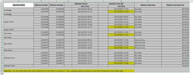
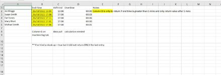
I need to build a new worksheet that returns only the last entry from a log sheet and to calculate overtime payments if the operator was still working 5 minutes after shift end.
I've tried a vlookup=true but that returns entries that are not the last ones in the sequence.
I've tried to upload the mini sheet but when I try and open it I get a message stating ' This file type is not supported in protective view' so I've had to upload images.
Thanks in advance for your help, as always.

 

[Legacy 143009]

An INDEXeption formula At least it will work Ops2 B2:

=OFFSET(INDEX(INDIRECT(ADDRESS(MATCH(A2,'Ops1'!$A$3:$A$25,0),7) &":$G$25"),MATCH(TRUE,INDEX(INDIRECT(ADDRESS(MATCH(A2,'Ops1'!$A$3:$A$25,0),7) &":$G$25")="",0),0)),-1,0)

Ops2 C2:

=FLOOR(B2, "1:00")

Ops2 D2:

=IF(C2-B2>=5,C2-B2,"00:00")

 

[ExceLoki]

part of the issue is the merged cells on ops1. excel is returning the value in the top cell reference only.
ex: 'ops1'!A3=Joe, 'ops1'!A3=0
you can unmerge those cells and fill them in with the same name, or copy and paste as formula, or maybe add a helper column.
in my solution i added a helper column
--------------

return max date-time, subtract times.xlsm
	A	B	C	D	E	F	G	H
1	operator name		machine#	machine#	machine track in		machine track out
2						start time		end time
3	Joe	Joe	12343549	12343549		10/26/22 8:59		10/26/22 11:19
4		Joe	12343549	12343549		10/26/22 11:34		10/26/22 13:04
5	Joe	Joe
6	Susan	Susan	12343646	12343646		10/26/22 9:03		10/26/22 9:03
7		Susan	12343646	12343646		10/26/22 9:11		10/26/22 10:37
8		Susan	12343646	12343646		10/26/22 10:55		10/26/22 12:33
9		Susan	12343646	12343646		10/26/22 13:04		10/26/22 15:05
10		Susan	12343646	12343646		10/26/22 15:26		10/26/22 17:08
11	Susan	Susan
12	Carl	Carl	12343659	12343659		10/26/22 8:59		10/26/22 14:31
13		Carl	12343659	12343659		10/26/22 11:34		10/26/22 17:11
14	Carl	Carl
15	Mary	Mary	12343579	12343579		10/26/22 8:59		10/26/22 11:02
16		Mary	12343579	12343579		10/26/22 11:34		10/26/22 13:29
17		Mary	12343579	12343579		10/26/22 8:59		10/26/22 15:53
18		Mary	12343579	12343579		10/26/22 11:34		10/26/22 17:01
19	Mary	Mary
20	Michael	Michael	12343677	12343677		10/26/22 8:59		10/26/22 10:47
21		Michael	12343677	12343677		10/26/22 11:34		10/26/22 12:39
22		Michael	12343677	12343677		10/26/22 8:59		10/26/22 13:00
23		Michael	12343677	12343677		10/26/22 8:59		10/26/22 15:17
24		Michael	12343677	12343677		10/26/22 11:34		10/26/22 17:06
25	Michael	Michael
ops1

----------------

return max date-time, subtract times.xlsm
	A	B	C	D
1		end time	shift end	overtime
2	Joe	10/26/22 13:04	13:00	0:00
3	Susan	10/26/22 17:08	17:00	0:08
4	Carl	10/26/22 17:11	17:00	0:11
5	Mary	10/26/22 17:01	17:00	0:00
6	Michael	10/26/22 17:06	17:00	0:06
ops2

Cell Formulas
Range	Formula
B2:B6	B2	=MAX(IF('ops1'!$B$3:$B$25=A2,'ops1'!$H$3:$H$25))
D2:D6	D2	=IF(TIME(HOUR(B2),MINUTE(B2),0)-TIME(HOUR(C2),MINUTE(C2),0)>0.00347222222626442,TIME(HOUR(B2),MINUTE(B2),0)-TIME(HOUR(C2),MINUTE(C2),0),0)

 

[Legacy 143009]

=OFFSET(INDEX(INDIRECT(ADDRESS(MATCH(A2,'Ops1'!$A$3:$A$25,0),7) &":$G$25"),MATCH(TRUE,INDEX(INDIRECT(ADDRESS(MATCH(A2,'Ops1'!$A$3:$A$25,0),7) &":$G$25")="",0),0)),-1,0)

A slightly shorter version would be:

=OFFSET(INDEX(INDIRECT("$G$"&MATCH(A2,'Ops1'!$A$3:$A$25,0) &":$G$25"),MATCH(TRUE,INDEX(INDIRECT("$G$"&MATCH(A2,'Ops1'!$A$3:$A$25,0) &":$G$25")="",0),0)),-1,0)

 

[harriet60]

An INDEXeption formula At least it will work Ops2 B2:

=OFFSET(INDEX(INDIRECT(ADDRESS(MATCH(A2,'Ops1'!$A$3:$A$25,0),7) &":$G$25"),MATCH(TRUE,INDEX(INDIRECT(ADDRESS(MATCH(A2,'Ops1'!$A$3:$A$25,0),7) &":$G$25")="",0),0)),-1,0)

Ops2 C2:

=FLOOR(B2, "1:00")

Ops2 D2:

=IF(C2-B2>=5,C2-B2,"00:00")

Thanks so much for taking the time to reply - it took a while to reposition the formulas into the work sheet but I got there! It is now working brilliantly -

 

[harriet60]

part of the issue is the merged cells on ops1. excel is returning the value in the top cell reference only.
ex: 'ops1'!A3=Joe, 'ops1'!A3=0
you can unmerge those cells and fill them in with the same name, or copy and paste as formula, or maybe add a helper column.
in my solution i added a helper column
--------------

return max date-time, subtract times.xlsm
	A	B	C	D	E	F	G	H
1	operator name		machine#	machine#	machine track in		machine track out
2						start time		end time
3	Joe	Joe	12343549	12343549		10/26/22 8:59		10/26/22 11:19
4		Joe	12343549	12343549		10/26/22 11:34		10/26/22 13:04
5	Joe	Joe
6	Susan	Susan	12343646	12343646		10/26/22 9:03		10/26/22 9:03
7		Susan	12343646	12343646		10/26/22 9:11		10/26/22 10:37
8		Susan	12343646	12343646		10/26/22 10:55		10/26/22 12:33
9		Susan	12343646	12343646		10/26/22 13:04		10/26/22 15:05
10		Susan	12343646	12343646		10/26/22 15:26		10/26/22 17:08
11	Susan	Susan
12	Carl	Carl	12343659	12343659		10/26/22 8:59		10/26/22 14:31
13		Carl	12343659	12343659		10/26/22 11:34		10/26/22 17:11
14	Carl	Carl
15	Mary	Mary	12343579	12343579		10/26/22 8:59		10/26/22 11:02
16		Mary	12343579	12343579		10/26/22 11:34		10/26/22 13:29
17		Mary	12343579	12343579		10/26/22 8:59		10/26/22 15:53
18		Mary	12343579	12343579		10/26/22 11:34		10/26/22 17:01
19	Mary	Mary
20	Michael	Michael	12343677	12343677		10/26/22 8:59		10/26/22 10:47
21		Michael	12343677	12343677		10/26/22 11:34		10/26/22 12:39
22		Michael	12343677	12343677		10/26/22 8:59		10/26/22 13:00
23		Michael	12343677	12343677		10/26/22 8:59		10/26/22 15:17
24		Michael	12343677	12343677		10/26/22 11:34		10/26/22 17:06
25	Michael	Michael
ops1

----------------

return max date-time, subtract times.xlsm
	A	B	C	D
1		end time	shift end	overtime
2	Joe	10/26/22 13:04	13:00	0:00
3	Susan	10/26/22 17:08	17:00	0:08
4	Carl	10/26/22 17:11	17:00	0:11
5	Mary	10/26/22 17:01	17:00	0:00
6	Michael	10/26/22 17:06	17:00	0:06
ops2

Cell Formulas
Range	Formula
B2:B6	B2	=MAX(IF('ops1'!$B$3:$B$25=A2,'ops1'!$H$3:$H$25))
D2:D6	D2	=IF(TIME(HOUR(B2),MINUTE(B2),0)-TIME(HOUR(C2),MINUTE(C2),0)>0.00347222222626442,TIME(HOUR(B2),MINUTE(B2),0)-TIME(HOUR(C2),MINUTE(C2),0),0)

Thank you also for taking the time to reply - your solution also works and I have been able to apply it to other spreadsheets so a double thanks for that - very grateful!

 

[Legacy 143009]

Dear @Fluff ,

I think @ExceLoki deserves the check mark more than me. It is much more simple and legible. Sometimes I got angry with myself for thinking way too complicated which makes me to miss such simple solutions. Also OP mentioned he will go for his solution. Regards..

I have been able to apply it to other spreadsheets