Looking up a partial match on a second table

[Rhewtani]

Okay, this is my first time asking a question in excel in 25 years. I've been able to figure out everything else.

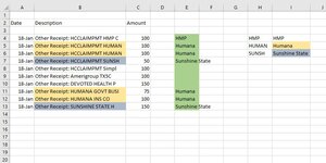
I've got data coming in from a bank feed. I want to look for key words in the description and match it with a table I have on a separate tab and get the xlookup result. For instance, if a cell contains the text "bcb" anywhere in it, I want it to look up bcb on the table and return "blue cross." In this way I'm mapping BCBS and BCBSF (each rows in that table) to blue cross.

Any ideas? The current process is memorizing all the possible codings and typing them into a manual field and having it look it up for me. There's often a string of numbers and letters before were the key words appear and it varies in length.

 

[eastrand]

You should be able to do something like this. If you want to post your data. We can give you an exact formula that will work for you.

=XLOOKUP("*bcb*",A1:A100,B1:B100,"no match",2)

Complements of Excel formula: XLOOKUP match text contains | Exceljet

 

[Rhewtani]

That definitely taught me something new. Here's an image of my exact issue. I want a formula in column E returning the result from the table in H:I on the match within the text in column B.

Make sense?

 

[eastrand]

Well, it's not an xlookup and definitely not the best way of doing it, but here is a solution. I don't think you can accomplish this with an xlookup.

Book1
	A	B	C	D	E	F	G	H	I
1
2	Date	Description	Amount
3
4	18-Jan	Other Receipt: HCCLAIMPMT HMP C	100		HMP			HMP	HMP
5	18-Jan	Other Receipt: HCCLAIMPMT HUMAN	100		Humana			HUMAN	Humana
6	18-Jan	Other Receipt: HCCLAIMPMT HUMAN	100		Humana			SUNSH	Sunshine State
7	18-Jan	Other Receipt: HCCLAIMPMT SUNSH	50		Sunshine State
8	18-Jan	Other Receipt: HCCLAIMPMT Simpl	100		No Match
9	18-Jan	Other Receipt: Amerigroup TX5C	100		No Match
10	18-Jan	Other Receipt: Devoted Health P	150		No Match
11	18-Jan	Other Receipt: HUMANA GOVT BUSI	75		Humana
12	18-Jan	Other Receipt: HUMANA INS CO	100		Humana
13	18-Jan	Other Receipt: SUNSHINE STATE H	150		Sunshine State
Sheet1

Cell Formulas
Range	Formula
E4:E13	E4	=IF(COUNTIF($B4,"*"&$H$4&"*"),$I$4,IF(COUNTIF($B4,"*"&$H$5&"*"),$I$5,IF(COUNTIF($B4,"*"&$H$6&"*"),$I$6,"No Match")))

 

[jtakw]

Hi,

See if this accomplishes what you need:

Book3.xlsx
	A	B	C	D	E	F	G	H	I
2	Date	Description	Amount
3
4	1/18/2022	Other Receipt: HCCLAIMPMT HMP C	100		HMP			HMP	HMP
5	1/18/2022	Other Receipt: HCCLAIMPMT HUMAN	100		Humana			HUMAN	Humana
6	1/18/2022	Other Receipt: HCCLAIMPMT HUMAN	100		Humana			SUNSH	Sunshine State
7	1/18/2022	Other Receipt: HCCLAIMPMT SUNSH	50		Sunshine State
8	1/18/2022	Other Receipt: HCCLAIMPMT Simpl	100		No Match
9	1/18/2022	Other Receipt: Amerigroup TX5C	100		No Match
10	1/18/2022	Other Receipt: Devoted Health P	150		No Match
11	1/18/2022	Other Receipt: HUMANA GOVT BUSI	75		Humana
12	1/18/2022	Other Receipt: HUMANA INS CO	100		Humana
13	1/18/2022	Other Receipt: SUNSHINE STATE H	150		Sunshine State
Sheet945

Cell Formulas
Range	Formula
E4:E13	E4	=IFERROR(LOOKUP(2,1/SEARCH(H$4:H$6,B4),I$4:I$6),"No Match")

EDIT NOTE: Just expand the H & I Column range sizes in the formula to fit your entire table.

 

[Fluff]

Another option

+Fluff 1.xlsm
	A	B	C	D	E	F	G	H	I
1
2	Date	Description	Amount
3
4	1/18/2022	Other Receipt: HCCLAIMPMT HMP C	100		HMP			HMP	HMP
5	1/18/2022	Other Receipt: HCCLAIMPMT HUMAN	100		Humana			HUMAN	Humana
6	1/18/2022	Other Receipt: HCCLAIMPMT HUMAN	100		Humana			SUNSH	Sunshine State
7	1/18/2022	Other Receipt: HCCLAIMPMT SUNSH	50		Sunshine State
8	1/18/2022	Other Receipt: HCCLAIMPMT Simpl	100
9	1/18/2022	Other Receipt: Amerigroup TX5C	100
10	1/18/2022	Other Receipt: Devoted Health P	150
11	1/18/2022	Other Receipt: HUMANA GOVT BUSI	75		Humana
12	1/18/2022	Other Receipt: HUMANA INS CO	100		Humana
13	1/18/2022	Other Receipt: SUNSHINE STATE H	150		Sunshine State
14
Lists

Cell Formulas
Range	Formula
E4:E13	E4	=FILTER($I$4:$I$6,ISNUMBER(SEARCH($H$4:$H$6,B4)),"")

 

[eastrand]

@Fluff, you always amaze me. The formulas I come up with work but when I come up with something like this

=IF(COUNTIF($B4,"*"&$H$4&"*"),$I$4,IF(COUNTIF($B4,"*"&$H$5&"*"),$I$5,IF(COUNTIF($B4,"*"&$H$6&"*"),$I$6,"No Match")))

You come up with this. Great job and so much simpler.

=FILTER($I$4:$I$6,ISNUMBER(SEARCH($H$4:$H$6,B4)),"")