Lookup a Match in an Array that can be in any column of the Array

[rehanahmad]

Hi
I am working on an Excel model where I am struggling to find a formula where I want to look for an exact match in a table of array that can be found in any columns out of 42 columns of the array with about 4000 rows. The search criteria I want to lookup can have up to 2 matches. Can someone please help?

 

[etaf]

what is you want to return , when you find that match ?
can you give some further examples

do you want to return the COLUMN Header or ROW header or both

something like this

GRID - Lookup Titles from a Value in the GRID.xlsx
	A	B	C	D	E	F	G	H
1		Title A	Title B	Title C		Criteria name
2	Object A	Tom	Pete	Dave		Phil
3	Object B	Ian	Mike	Phil		Expected result
4	Object C	Gary	Andre	Kevin		Object B-Title C		INDEX(A2:A4,MIN(IF(B2:D4=F2,ROW(A2:A4)-ROW(A2)+1)))&"-"&INDEX($B$1:$D$1,MIN(IF(B2:D4=F2,COLUMN(B2:D2)-COLUMN(B2)+1)))
5								Need Control+Shift+Enter - array formula
6
7								Find the Row and Column info based on the cell in the Grid
8
9
10			FIND Phil		ROW	Object B	= >>	INDEX(A2:A4,MIN(IF(B2:D4=F2,ROW(A2:A4)-ROW(A2)+1)))
11
12			Find Phil		COLUMN	Title C	= >>	INDEX($B$1:$D$1,MIN(IF(B2:D4=F2,COLUMN(B2:D2)-COLUMN(B2)+1)))
13
Sheet1

Cell Formulas
Range	Formula
F4	F4	=INDEX(A2:A4,MIN(IF(B2:D4=F2,ROW(A2:A4)-ROW(A2)+1)))&"-"&INDEX($B$1:$D$1,MIN(IF(B2:D4=F2,COLUMN(B2:D2)-COLUMN(B2)+1)))
F10	F10	=INDEX(A2:A4,MIN(IF(B2:D4=F2,ROW(A2:A4)-ROW(A2)+1)))
F12	F12	=INDEX($B$1:$D$1,MIN(IF(B2:D4=F2,COLUMN(B2:D2)-COLUMN(B2)+1)))
Press CTRL+SHIFT+ENTER to enter array formulas.

 

[Peter_SSs]

I suggest that you update your Account details (or click your user name at the top right of the forum) so helpers always know what Excel version(s) & platform(s) you are using as the best solution often varies by according to that information. (Don’t forget to scroll down & ‘Save’)

 

[rehanahmad]

Hi thanks for your prompt reply.
What I got is two sheets, one of them is a table as shown in Table 1.
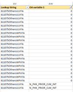
Other one has got some data (Table 2) where I want to lookup the string in AV to match with any columns from T:AH....... and return me Column B (OA Variable) in Table 1.
A match can have up to 3 values in column B which I want to returns in different columns.
Trust this helps.
Many thanks for your help.

 

[Peter_SSs]

Any possibility of addressing the issue that I raised?

 

[rehanahmad]

Any possibility of addressing the issue that I raised?

Hi I have updated
Thanks

 

[Peter_SSs]

Hi I have updated
Thanks

Thanks. See if you can adapt this (with Excel 2019) to your layout/sheet names if it does what you want.

rehanahmad.xlsm
	A																			T	U	V	W	X	Y	Z	AA	AB
1	OA Variable																			Hdr2	Hdr3	Hdr4	Hdr5	Hdr6	Hdr7	Hdr8	Hdr9	Hdr10
2	A																			K1	Y9	I2	X8	Q4	G8	A8	D8	Y5
3	B																			P2	U8	P8	D5	I7	I7	K4	W4	Y9
4	C																			E2	W4	O5	B8	W8	Q1	E5	T4	F4
5	D																			G6	B2	O3	A3	Y9	J5	F2	Z5	K5
Sheet1

rehanahmad.xlsm
	A	B	C	D
1	Lookup String	Result 1	Result 2	Result 3
2	W4	B	C
3	A6
4	Y9	A	B	D
5	K9
6	J5	D
7	O3	D
Sheet2

Cell Formulas
Range	Formula
B2:D7	B2	=IFERROR(INDEX(FILTERXML("<p><c>"&TEXTJOIN("</c><c>",1,INDEX(Sheet1!$A:$A,IF(Sheet1!$T$2:$AB$5=$A2,ROW(Sheet1!$A$2:$A$5),99))&"")&"</c></p>","//c"),COLUMNS($B:B)),"")

If you want helpers to work with your actual sample data and layout, investigate XL2BB for providing small dummy sample data and expected results.

 

[rehanahmad]

IFERROR(INDEX(FILTERXML("<p><c>"&TEXTJOIN("</c><c>",1,INDEX(Sheet1!$A:$A,IF(Sheet1!$T$2:$AB$5=$A2,ROW(Sheet1!$A$2:$A$5),99))&"")&"</c></p>","//c"),COLUMNS($B:B)),"")

Hi Many thanks for looking into. I have applied your logic but all cells returning blank. Can i please ask what "<p><c>" represent? and also if this formula will only work with xlsm version?

 

[Peter_SSs]

Hi Many thanks for looking into. I have applied your logic but all cells returning blank.

Sounds like either you have not applied it correctly or else there is something significantly different about your data and my sample data.
If you have XL2BB installed then perhaps you could provide a small set of dummy sample data that we can test with.

Also, if you start a new workbook you could test with my sample data (depending on the outcome of my final point below). Copy my Sheet1 sample data to cell A1 of your Sheet1 by using this button at the top left of my mini-sheet

Then repeat with my Sheet2

Can i please ask what "<p><c>" represent?

There is nothing special about them being p and c but they are to ensure that the string being processes by the FILTERXML function is a valid XML string.

also if this formula will only work with xlsm version?

No, the formula does not need to be in an xlsm workbook but it does require Excel 2013 or later (which your profile update shows you have) and a Windows platform, not Mac, (which unfortunately did not get updated in your profile)

.. so helpers always know what Excel version(s) & platform(s) you are using ..

 

[rehanahmad]

Hi peter, I am working on it,
part of the formula "COLUMNS($B:B))", is it referring to the Column B where the formula is written? i.e. if the formula is written in B2 in your example, it this part "COLUMNS($B:B))" referring to the same column?