Lookup and calculate value based on status and date in a range

[NikShah]

Hi,

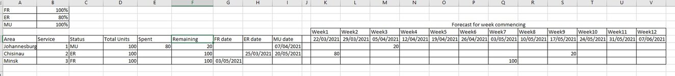
I am trying to calculate a value based on the remaining units (Col F) which is dependent on the status (Col C) that also is dependant on a date in the appropriate column (Cols G to I).

For example; if the status is MU then 100% (cell B3) of the remainder (cell F6) is calculated and the correct date - in this case - Col I is referenced and the value is placed in forecast box in the appropriate week.

It gets more complicated when the status is ER as 80% is calculated for one week and the remaining 20% in another week specified in Col G to I.

Please see screenshot below for the desired result.

Many thanks in advance!

Regards,

 

[NikShah]

I tried to use the following formulas and each of them works in isolation, but I just cannot seem to combine them!

=IF($C6="MU",IF(AND($I6>=K$5,$I6<L$5),($F6*VLOOKUP($C6,$A$1:$B$3,2,0)),0))
=IF($C7="ER",IF(AND($H7>=K$5,$H7<L$5),($F7*VLOOKUP($C7,$A$1:$B$3,2,0)),IF(AND($I7>=K$5,$I7<L$5),($F7*(1-VLOOKUP($C7,$A$1:$B$3,2,0))),0)))
=IF($C8="FR",IF(AND($G8>=K$5,$G8<L$5),($F8*VLOOKUP($C8,$A$1:$B$3,2,0)),0))

 

[Peter_SSs]

A couple of suggestions that should help get you better/faster responses for any future question:

1. Update your Account details (click your user name at the top right of the forum) so helpers always know what Excel version(s) & platform(s) you are using as the best solution often varies by version. (Don’t forget to scroll down & ‘Save’)
   
   
2. Investigate XL2BB for providing sample data to make it easier for helpers by not having to manually type out sample data to test with.

See if this does what you want. It assumes column J is blank as in your image.

NikShah.xlsm
	A	B	C	D	E	F	G	H	I	J	K	L	M	N	O	P	Q	R	S	T	U	V
1	FR	100%
2	ER	80%
3	MU	100%
4
5						Remaining	FR date	ER date	MU date		22/03/2021	29/03/2021	5/04/2021	12/04/2021	19/04/2021	26/04/2021	3/05/2021	10/05/2021	17/05/2021	24/05/2021	31/05/2021	7/06/2021
6			MU			20			7/04/2021				20
7			ER			100		25/03/2021	20/05/2021		80								20
8			FR			100	3/05/2021										100
Sheet1

Cell Formulas
Range	Formula
K6:V8	K6	=IF(LOOKUP(MIN($G6:$I6),$K$5:$V$5)=K$5,$F6*VLOOKUP($C6,$A$1:$B$3,2,0),IF(AND($C6="ER",LOOKUP(MAX($G6:$I6),$K$5:$V$5)=K$5),$F6-SUM($J6:J6),""))

 

[NikShah]

Hi Peter,

Apologies for the delay. I couldn't download the XL2BB add on as this is a company computer.

Your solution is way more elegant than mine and works!

If you delete column J then I get the following solution for cell J6:

=IF($C6="MU",IF(AND($I6>=J$5,$I6<K$5),($F6*VLOOKUP($C6,$A$1:$B$3,2,0)),0),
IF($C6="ER",IF(AND($H6>=J$5,$H6<K$5),($F6*VLOOKUP($C6,$A$1:$B$3,2,0)),IF(AND($I6>=J$5,$I6<K$5),($F6*(1-VLOOKUP($C6,$A$1:$B$3,2,0))),0)),
IF($C6="FR",IF(AND($G6>=J$5,$G6<K$5),($F6*VLOOKUP($C6,$A$1:$B$3,2,0)),0),0)))

Thank you once again.

 

[Peter_SSs]

If you delete column J then I get the following solution for cell J6:

=IF($C6="MU",IF(AND($I6>=J$5,$I6<K$5),($F6*VLOOKUP($C6,$A$1:$B$3,2,0)),0),
IF($C6="ER",IF(AND($H6>=J$5,$H6<K$5),($F6*VLOOKUP($C6,$A$1:$B$3,2,0)),IF(AND($I6>=J$5,$I6<K$5),($F6*(1-VLOOKUP($C6,$A$1:$B$3,2,0))),0)),
IF($C6="FR",IF(AND($G6>=J$5,$G6<K$5),($F6*VLOOKUP($C6,$A$1:$B$3,2,0)),0),0)))

If column J is deleted, then you could use this slightly adjusted version of my previous formula

NikShah.xlsm
	A	B	C	D	E	F	G	H	I	J	K	L	M	N	O	P	Q	R	S	T	U
1	FR	100%
2	ER	80%
3	MU	100%
4
5						Remaining	FR date	ER date	MU date	22/03/2021	29/03/2021	5/04/2021	12/04/2021	19/04/2021	26/04/2021	3/05/2021	10/05/2021	17/05/2021	24/05/2021	31/05/2021	7/06/2021
6			MU			20			7/04/2021			20
7			ER			100		25/03/2021	20/05/2021	80								20
8			FR			100	3/05/2021									100
Sheet3

Cell Formulas
Range	Formula
J6:U8	J6	=IF(LOOKUP(MIN($G6:$I6),$J$5:$U$5)=J$5,$F6*VLOOKUP($C6,$A$1:$B$3,2,0),IF(AND($C6="ER",LOOKUP(MAX($G6:$I6),$J$5:$U$5)=J$5),$F6-SUM($I6:I6)+$I6,""))

 

[NikShah]

If you enter a date in cell H6, say, 23/3/21, then the formula doesn't work as it will enter a value in cell J6 instead of the correct cell L6. Basically what I'm trying to say that in the past we would have had an early release date, but it's the status that should be driving which date column should be picked up.

 

[Peter_SSs]

OK, now I understand (I think! ). From your previous example and description I thought it was only "ER" rows that would have two dates.

See if this is better.

NikShah.xlsm
	A	B	C	D	E	F	G	H	I	J	K	L	M	N	O	P	Q	R	S	T	U
1	FR	100%
2	ER	80%
3	MU	100%
4
5						Remaining	FR date	ER date	MU date	22/03/2021	29/03/2021	5/04/2021	12/04/2021	19/04/2021	26/04/2021	3/05/2021	10/05/2021	17/05/2021	24/05/2021	31/05/2021	7/06/2021
6			MU			20		23/03/2021	7/04/2021			20
7			ER			100		25/03/2021	20/05/2021	80								20
8			FR			100	3/05/2021									100
Sheet4

Cell Formulas
Range	Formula
J6:U8	J6	=IF(LOOKUP(INDEX($G6:$I6,MATCH($C6&"*",$G$5:$I$5,0)),$J$5:$U$5)=J$5,$F6*VLOOKUP($C6,$A$1:$B$3,2,0),IF(AND($C6="ER",LOOKUP(MAX($G6:$I6),$J$5:$U$5)=J$5),$F6-SUM($I6:I6)+$I6,""))

 

[NikShah]

Are you able to advise what this part of the formula is doing? At the moment it's not adding anything from the date column (Col I).

 

[Peter_SSs]

Are you able to advise what this part of the formula is doing? At the moment it's not adding anything from the date column (Col I).

We don't want it to add anything from the date column. That part of the formula is like that so that we can use the same formula in all columns. If we had a separate formula for column J then another formula for all the other columns we wouldn't need that part of the formula to be quite like that. That part of the formula is to calculate the second value in the "ER" rows like in cell R7 in my sheet above. In that cell, that part of the formula you marked is
$F7-SUM($I7:Q7)+$I7
It sums all the values from I7:Q7 and subtracts that from F7 (100). However, the sum that was subtracted includes the date from I7 which should not be subtracted so it is added back on at the end. This results in the 20 you see in R7.

 

[NikShah]

We don't want it to add anything from the date column. That part of the formula is like that so that we can use the same formula in all columns. If we had a separate formula for column J then another formula for all the other columns we wouldn't need that part of the formula to be quite like that. That part of the formula is to calculate the second value in the "ER" rows like in cell R7 in my sheet above. In that cell, that part of the formula you marked is
$F7-SUM($I7:Q7)+$I7
It sums all the values from I7:Q7 and subtracts that from F7 (100). However, the sum that was subtracted includes the date from I7 which should not be subtracted so it is added back on at the end. This results in the 20 you see in R7.

Ah ok. Understood. Thanks again.