Lookup and subtract

[milesy]

HI all

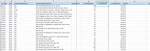
im after some help to solve an issue i have a spreasheet that looks like the below image

what i need to do is a script that will look at Column C and in the first instance return the value of Column H into say Column Z
then for the NEXT instance of the same value in Column C return the result of Z- the new value of H

So for the below example
C00684 first instance Z would be 76 - Column H (20) so 56
Second instance of C00684 would be Z(56) subtracting the new value of I (in this instance 50 ) so Z on row 81 would be 6
etc etc etc

any one care to help here?

 

[Fluff]

How about
=INDEX($I$2:$I$100,MATCH(C2,$C$2:$C$100,0))-SUMIFS($H$2:$H$100,$C$2:$C$100,C2)

 

[milesy]

interesting looks close but not quite right.....

i think this works based on your suggestion

=INDEX($I$2:$I1705,MATCH(C1705,$C$2:$C1705,0))-SUMIFS($H$2:$H1705,$C$2:$C1705,C1705)

 

[Fluff]

That looks to be exactly the same formula, just looking at a different cell.

Glad it's sorted & thanks for the feedback.

 

[milesy]

lol actually the change was simply to remove the abosolute settings on the match....what it was doing (which wasnt quite what i wanted) was subtracting all the quantites at once rather than a starting piont....then subtract each value as it went
either way thank you so much for your help

 

[Fluff]

Got it, & thanks for the feedback.

 

[milesy]

Can i ask you (or anyone else who might know) ......with the above formula i would like to be able to run a macro which would basically ask me for the columns that apply

what i mean is from the code above there are four sections

INDEX($I$2:$I2,MATCH(C2,$C$2:$C2,0))-SUMIFS($H$2:$H2,$C$2:$C2,C2)

the first section in this instance is Column I, the second Column C the third H and the final C

so i would want a macro (or script) to pop up and ask me
1. Where to paste the finished result,
2 which column is the Qty on hand (Column I),
3. which columns is the Part Number (Column C)
4. Which Column is the used qty (Column H)

and then paste the final formula with the details filled in, this would make this report and the responding code very very usable?

Adrian

 

[Fluff]

As that is a totally different question, you will need to start a new thread. Thanks