Lookup based on two criteria

anuradhagrewal

Board Regular
Joined
Dec 3, 2020
Messages
85
Office Version
  1. 2010
Platform
  1. Windows
Hello
I have a problem.
I have two tables in Sheet 1 and Sheet 2 of a workbook.
There are 3 fields in each of the tables out of which Name and Date are common in both the worksheets with varying data.
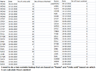
Now I want to function which matches the name and date with the hours worked on that date by that person.
For eg : WDAU (A2) on 6-Dec-20 (B2) sold 22 units (C3) then on the given date how many hours did he work which is to be picked from sheet 2.
The same name can sell on different dates different units and work for different hours.
This all needs to be matched into a single table.
I have tried Vlookup(A2&B2 sheet2!A2:C40,3,false) but it return #N/A.
Can anybody please help. As always it will be much appreciated.

Thanks in advance

Regards

Anu
 

Attachments

  • tabel.png
    tabel.png
    42.9 KB · Views: 14

Excel Facts

Copy formula down without changing references
If you have =SUM(F2:F49) in F50; type Alt+' in F51 to copy =SUM(F2:F49) to F51, leaving the formula in edit mode. Change SUM to COUNT.
Hi Anuradhagrewal,

To use VLOOKUP you'd need to add a worker column with the table_array as a concatenated Name and Date from the searched on sheet and the lookup_value as the concatenated Name and Date as you have shown.

You could also do this using INDEX/MATCH/INDEX or INDEX/AGGREGATE without using a worker column.

It would be best if you could upload your data with a worked example using XL2BB, or even as a text table, so people don't have to type lots of test data.
 
Upvote 0
Thanks for your reply....
But i would much appreciate if you can share with me the exact formula for the one mentioned.
Once again thank u for your time.
 
Upvote 0
I'm not going to type your data so here's a sample using my test data:

Anuradhagrewal.xlsx
ABCDEFGHIJ
1NameDateUnits SoldHours WorkedWorker ColumnNameDateHours Worked
2Fred1/1/202077:12Fred43831Fred1/1/20207:12
3Fred1/2/202048:55Jim43831Jim1/1/20208:47
4Fred1/4/202039:44Fred43832Fred1/2/20208:55
5Fred1/6/2020227:22Jim43833Jim1/3/20209:36
6Jim1/1/202038:47Fred43834Fred1/4/20209:44
7Jim1/3/202089:36Jim43835Jim1/5/20208:12
8Jim1/5/202018:12Fred43836Fred1/6/20207:22
9Jim1/6/202029:23Jim43836Jim1/6/20209:23
Sheet1
Cell Formulas
RangeFormula
D2:D9D2=VLOOKUP(A2&B2,$G$2:$J$9999,4,0)
G2:G9G2=H2&I2
 
Upvote 0
In this case there's no need for VLOOKUP, something like this should work

=SUMIFS(Sheet2!C:C, Sheet2!A:A, "WDAU", Sheet2!B:B, DateValue("6-14-2020"))
 
Upvote 0

Forum statistics

Threads
1,214,918
Messages
6,122,243
Members
449,075
Latest member
staticfluids

We've detected that you are using an adblocker.

We have a great community of people providing Excel help here, but the hosting costs are enormous. You can help keep this site running by allowing ads on MrExcel.com.
Allow Ads at MrExcel

Which adblocker are you using?

Disable AdBlock

Follow these easy steps to disable AdBlock

1)Click on the icon in the browser’s toolbar.
2)Click on the icon in the browser’s toolbar.
2)Click on the "Pause on this site" option.
Go back

Disable AdBlock Plus

Follow these easy steps to disable AdBlock Plus

1)Click on the icon in the browser’s toolbar.
2)Click on the toggle to disable it for "mrexcel.com".
Go back

Disable uBlock Origin

Follow these easy steps to disable uBlock Origin

1)Click on the icon in the browser’s toolbar.
2)Click on the "Power" button.
3)Click on the "Refresh" button.
Go back

Disable uBlock

Follow these easy steps to disable uBlock

1)Click on the icon in the browser’s toolbar.
2)Click on the "Power" button.
3)Click on the "Refresh" button.
Go back
Back
Top