Lookup for MULTIPLE values and return a specific cell if AT LEAST ONE criteria is met

[simonesk]

Dear all,

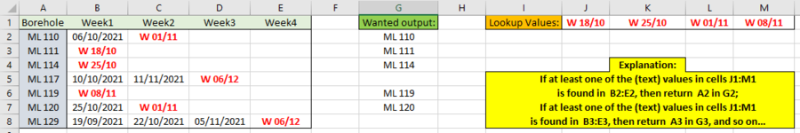
I am trying to find a specific value (from multiple options) in an array (Please, see the picture below). I tried several formulas, playing with OR, HLOOKUP, INDEX and MATCH, but I couldn't find a working formula yet. It is all good if I look for a single value, but as soon as I add multiple criteria I get #VALUE or #N/A, or similar errors.

Could you be so kind to help me out with this matter?

Regards,

Simone

MyData:

Borehole Week1 Week2 Week3 Week4 Wanted output: Lookup Values: W 18/10 W 25/10 W 01/11 W 08/11
ML 110 06/10/2021 W 01/11 ML 110
ML 111 W 18/10 ML 111
ML 114 W 25/10 ML 114
ML 117 10/10/2021 11/11/2021 W 06/12
ML 119 W 08/11 ML 119
ML 120 25/10/2021 W 01/11 ML 120
ML 129 19/09/2021 22/10/2021 05/11/2021 W 06/12

 

[RasGhul]

Hi Simone,

Maybe this, drag down the array far enough to return total count.

Book1
	A	B	C	D	E	F	G	H	I	J	K	L	M	N
1	Borehole	Week1	Week2	Week3	Week4		Output	Count		Values	w 18/10	w 25/10	w 01/11	w 08/11
2	ML110	6/10/2021	W 01/11				ML110	5
3	ML111	W 18/10					ML111
4	ML114	W 25/10					ML114
5	ML117	10/10/2021	11/11/2021	W 06/12			ML119
6	ML119	W 08/11					ML120
7	ML120	25/10/2021	W 01/11
8	ML129	19/09/2021	22/10/2021	5/11/2021	W 06/12
Sheet1

Cell Formulas
Range	Formula
H2	H2	=SUMPRODUCT(($B$2:$E$8=K1)+($B$2:$E$8=L1)+($B$2:$E$8=M1)+($B$2:$E$8=N1))
G2:G8	G2	=IF(ROWS($G$2:G2)>$H$2,"",INDEX($A$2:$A$8,SMALL(IF(($B$2:$E$8=$K$1)+($B$2:$E$8=$L$1)+($B$2:$E$8=$M$1)+($B$2:$E$8=$N$1),ROW($A$2:$A$8)-ROW($A$1)),ROWS($G$2:G2))))
Press CTRL+SHIFT+ENTER to enter array formulas.

 

[Fluff]

Another option

+Fluff 1.xlsm
	A	B	C	D	E	F	G	H	I	J	K	L	M
1	Borehole	Week1	Week2	Week3	Week4		Output		Values	w 18/10	w 25/10	w 01/11	w 08/11
2	ML110	06/10/2021	W 01/11				ML110
3	ML111	W 18/10					ML111
4	ML114	W 25/10					ML114
5	ML117	10/10/2021	11/11/2021	W 06/12
6	ML119	W 08/11					ML119
7	ML120	25/10/2021	W 01/11				ML120
8	ML129	19/09/2021	22/10/2021	05/11/2021	W 06/12
9
Main

Cell Formulas
Range	Formula
G2:G8	G2	=IF(SUM(COUNTIFS(B2:E2,$J$1:$M$1)),A2,"")