Lookup max value that meets all criteria

[Drew_]

Hi all.

I have a fairly complicated question and I've been racking my brain for a while. I have the following data set:

<style type="text/css"><!--td {border: 1px solid #ccc;}br {mso-data-placement:same-cell;}--></style>

	Drew	Ruben	Hussain	Push Ups	Sit Ups	Week Ending Date
50% Normal for Week?	Yes	No	Yes	200	250	4/1/18
10% Triangle for Week?	Yes	Yes	Yes	575	25	4/1/18
20% Wide for Week?	No	Yes	Yes	225	0	4/1/18
50% Normal for Week?	No	No	No			4/8/18
10% Triangle for Week?	No	No	No			4/8/18
20% Wide for Week?	No	No	No			4/8/18
50% Normal for Week?	No	No	No			4/15/18
10% Triangle for Week?	No	No	No			4/15/18
20% Wide for Week?	No	No	No			4/15/18
50% Normal for Week?	No	No	No			4/22/18
10% Triangle for Week?	No	No	No			4/22/18
20% Wide for Week?	No	No	No			4/22/18
50% Normal for Week?	No	No	No			4/29/18
10% Triangle for Week?	No	No	No			4/29/18
20% Wide for Week?	No	No	No			4/29/18

<colgroup><col style="width: 146px"><col width="79"><col width="83"><col width="73"><col width="58"><col width="58"><col width="84"></colgroup><tbody>
</tbody>

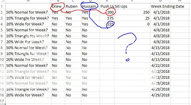
Drew has 200 push ups, Ruben has 575, and Hussain has 225. Essentially, I want to return the name of the person who has the maximum number of push ups AND who meets all 3 criteria (3 Yes') for each date. So I need to come up with a formula that will return "Hussain" as my answer.

I've tried various MAX/IF functions, INDEX/MATCH variables, SUMPRODUCT formulas, and I think I just have too many criteria. Or maybe I need to organize my data better (probably this).

Any help would be appreciated. Thank you.

 

[dave2018]

Hi, i'm not sure how the pushup values correspond to the names. and does column A have to do with this?

 

[Drew_]

Yes, I figured I needed to reorganize my data. The push up values don't correspond to the names as of now, I was not sure how to include them in the table.

Essentially, I am doing a competition with my buddies and we are seeing who can do the most push ups in a week, and we're doing it every week for a few months. I want to label a winner each week; however, the winner must meet all 3 criteria, which are 50% of their reps have to be normal push ups, 10% of the reps have to be triangle push ups and 20% of the reps have to be wide angle push ups. So what I want my formula to say is this:

"Tell me who did the most push ups this week AND met all 3 criteria." So even though Ruben has completed 575 push ups, he has not met all 3 criteria therefore he can't win.

 

[Drew_]

I transposed my column headers so I think this will work better:

<style type="text/css"><!--td {border: 1px solid #ccc;}br {mso-data-placement:same-cell;}--></style>

	50% Normal for Week?	10% Triangle for Week?	20% Wide for Week?	Push Ups	Sit Ups	Week Ending Date
Drew	Yes	Yes	No	200	250	4/1/18
Ruben	Yes	No	Yes	575	50	4/1/18
Hussain	Yes	Yes	Yes	225	0	4/1/18
Drew	No	No	No			4/8/18
Ruben	No	No	No			4/8/18
Hussain	No	No	No			4/8/18
Drew	No	No	No			4/15/18
Ruben	Yes	No	No			4/15/18
Hussain	No	No	No			4/15/18
Drew	No	No	No			4/22/18
Ruben	No	No	No			4/22/18
Hussain	No	No	No			4/22/18

<colgroup><col style="width: 54px"><col width="79"><col width="83"><col width="73"><col width="58"><col width="58"><col width="84"></colgroup><tbody>
</tbody>

I have the following formula that tells me the name of the MAX for the week: INDEX($R$3:$R$5,MATCH(MAX(V3:V5),V3:V5,0)) where the names are in the R column. However, this formula does not consider the criteria, and I need all 3 criteria to say "Yes" in order for a winner to be determined.

 

[Eric W]

Something like this?

	A	B	C	D	E	F	G	H	I	J
1		50% Normal for Week?	10% Triangle for Week?	20% Wide for Week?	Push Ups	Sit Ups	Week Ending Date		Week	Winner
2	Drew	Yes	Yes	No	200	250	4/1/2018		4/1/2018	Hussain
3	Ruben	Yes	No	Yes	575	50	4/1/2018		4/8/2018	Drew
4	Hussain	Yes	Yes	Yes	225	0	4/1/2018		4/15/2018	No one
5	Drew	Yes	Yes	Yes	250		4/8/2018		4/22/2018	Hussain
6	Ruben	No	No	No	275		4/8/2018
7	Hussain	No	No	No	300		4/8/2018
8	Drew	Yes	Yes	No	100		4/15/2018
9	Ruben	Yes	No	Yes	125		4/15/2018
10	Hussain	No	Yes	Yes	250		4/15/2018
11	Drew	No	No	No	300		4/22/2018
12	Ruben	Yes	Yes	Yes	123		4/22/2018
13	Hussain	Yes	Yes	Yes	444		4/22/2018

<colgroup><col style="width: 25pxpx"><col><col><col><col><col><col><col><col><col><col></colgroup><thead>
</thead><tbody>
</tbody>

Sheet1​

Array Formulas Cell Formula J2 {=IFERROR(INDEX(A:A,MOD(LARGE(IF(MMULT(IF($B$2:$D$13="Yes",1,0),{1;1;1})=3,IF($G$2:$G$13=I2,$E$2:$E$13+ROW($E$2:$E$13)/10000)),1),1)*10000),"No one")} <thead> </thead><tbody> </tbody> Entered with Ctrl+Shift+Enter. If entered correctly, Excel will surround with curly braces {}. Note: Do not try and enter the {} manually yourself

<tbody>
</tbody>

 

[Drew_]

Yes this works amazingly! Thank you so much.