Lookup

[J_Kelly]

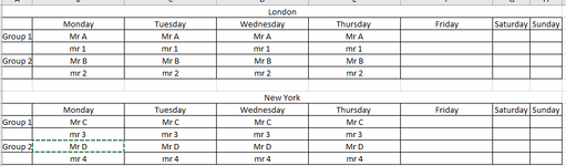
I have a multiple tables of data similar to the screenshot attached. I am trying to lookup and bring back the area the group is in i.e. London. The tables vary from having 1 group to 30 groups and there are at least 20 areas.

I am trying to lookup against Mr A to bring back that he is in London on a separate sheet.

I thought maybe Hlookup or Xlookup but trying to incorporate an if statement doesnt seem to work. I get a new sheet every week but it is always in the same format just with varying numbers of groups.

The final product I am trying to get to is this, just so at a quick glance since I deal group by group I can see where they are as that affects different processes

 

[GlennJ]

You could do it with an IF Statement, but the formula would be large. Probably a better way to do it. But this would work.

=IF(B3=Sheet1!$B$3,Sheet1!$A$1, IF(B3=Sheet1!$B$4,Sheet1!$A$1, IF(B3=Sheet1!$B$5,Sheet1!$A$1, IF(B3=Sheet1!$B$6,Sheet1!$A$1, IF(B3=Sheet1!$B$9,Sheet1!$A$8, IF(B3=Sheet1!$B$10,Sheet1!$A$8, IF( B3=Sheet1!$B$11,Sheet1!$A$8, IF(B3=Sheet1!$B$12,Sheet1!$A$8,""))))))))

This would have to be expanded to cover all 30 groups and it assumes that each person is at the location on Monday and stays there all week. Formula goes in Sheet 2, Cell C3 and can be dragged down, once expanded.

 

[J_Kelly]

That's the biggest issue is that its all delimited week in week out the formula using IF would be infinitely long, I found =INDEX(A:A,MATCH("Group 1",A:A,0)-1,,1) which return the location however it only returns the first instance of it. I thought of having a blank column because then I am able to just Vlookup against the list of people, so after the Sundat column I can just have a hidden column that lists out the location. So next to London you would have 5 instances of 'London' in column I, an error in row 7 then 'New York' would appear and so on.

This is the easiest option I can think of to assign a column for a location list and then vlookup the names against the list versus trying to do everything in one instance

 

[J_Kelly]

You could do it with an IF Statement, but the formula would be large. Probably a better way to do it. But this would work.

View attachment 80898View attachment 80899

=IF(B3=Sheet1!$B$3,Sheet1!$A$1, IF(B3=Sheet1!$B$4,Sheet1!$A$1, IF(B3=Sheet1!$B$5,Sheet1!$A$1, IF(B3=Sheet1!$B$6,Sheet1!$A$1, IF(B3=Sheet1!$B$9,Sheet1!$A$8, IF(B3=Sheet1!$B$10,Sheet1!$A$8, IF( B3=Sheet1!$B$11,Sheet1!$A$8, IF(B3=Sheet1!$B$12,Sheet1!$A$8,""))))))))

This would have to be expanded to cover all 30 groups and it assumes that each person is at the location on Monday and stays there all week. Formula goes in Sheet 2, Cell C3 and can be dragged down, once expanded.

Apologies I was supposed to post the reply I sent in response to this.

=INDEX(A:A,MATCH(Sheet1!B3,B:B,0)-1,,1) I thought about using this which worked for the first instance however it only works if the name appears against Group 1, I thought about adding an IF statement and the false value being a follow up if statement to removing varying increments dependent on the group number i.e. Group 1 is -1, Group 2 is -3, Group 3 is -5 and so on, this however only gave me a FALSE error even against Mr A when it technically meets the true condition.