Loop through Rows and Return Non-Blank Cells Based on Column Headers [VBA]

[eda]

Hi,

I've seen some similar questions but not quite what I need asked before, any help or suggestions would be greatly appreciated.

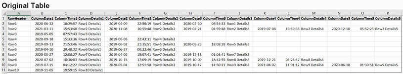
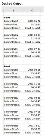
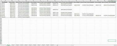
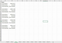
I have multiple rows that contain column headers with the same name (but for a number added on to the end), what I’d like to do is to loop through each row and column and output the row data so only non-blank cells relevant to the header name are returned. I've attached an image of the original table and also the desired output as hopefully this will provide a clearer idea as to what I'd like to achieve.

Many thanks in advance.

 

[Crystalyzer]

How many columns are in the original data?
where do you want the output? New worksheet? New Workbook?

Please post a sample of the data using XL2BB (See signature for instructions)

 

[Peter_SSs]

Welcome to the MrExcel board!

Try this with a copy of your workbook.
This puts the results on the same worksheet as the original data but off to the right.

Sub Rearrange()
  Dim a As Variant, b As Variant
  Dim i As Long, j As Long, k As Long, uba2 As Long, nr As Long
  
  With Range("A1").CurrentRegion
    a = .Value2
    uba2 = UBound(a, 2)
    nr = 1
    ReDim b(1 To Rows.Count, 1 To 2)
    For i = 2 To UBound(a)
      nr = nr + 1
      b(nr, 1) = a(i, 1)
      nr = nr + 1
      For j = 2 To uba2 Step 3
        If IsEmpty(a(i, j)) Then
          Exit For
        Else
          For k = 0 To 2
            b(nr + k, 1) = a(1, j + k)
            b(nr + k, 2) = a(i, j + k)
          Next k
          nr = nr + 4
        End If
      Next j
    Next i
    .Offset(, uba2 + 3).Resize(nr, 2).Value = b
  End With
End Sub

 

[DanteAmor]

Hi and welcome to MrExcel.

Here is another macro for you to consider.

The source data on sheet1, the output on sheet2.

Sub Loop_Rows2()
  Dim sh1 As Worksheet, sh2 As Worksheet
  Dim i As Long, j As Long, k As Long
  Set sh1 = Sheets("Sheet1")    'Data
  Set sh2 = Sheets("Sheet2")    'Output
  sh2.Range("B:C").Clear
  k = 1
  For i = 2 To sh1.Range("A" & Rows.Count).End(3).Row
    k = k + 1
    sh2.Range("B" & k).Value = sh1.Range("A" & i).Value
    k = k + 1
    For j = 2 To sh1.Cells(i, Columns.Count).End(1).Column Step 3
      sh2.Range("B" & k).Resize(3, 2).Value = Application.Transpose(Array(sh1.Cells(1, j).Resize(1, 3), sh1.Cells(i, j).Resize(1, 3)))
      k = k + 4
    Next
  Next
End Sub

 

[eda]

Hi Peter_SSs and DanteAmor, thank you so much for the warm welcome to the MrExcel board and for the brilliant macro’s, they are exactly what I wanted and work perfectly!

Thank you for observing the output to be displayed to the right of the data on the same worksheet or on Sheet2 respectively. What I would really like to do with the output is to loop through and display in separate Worksheets based on Sheet1’s Row Number (please see the images for hopefully a clearer idea), any help or suggestions would be greatly appreciated and apologies for not outlining the output destination in my original post.

Many thanks again in advance.

 

[DanteAmor]

Try this:

Sub Loop_Rows2()
  Dim sh1 As Worksheet
  Dim i As Long, j As Long
  Dim sName As String
  
  Application.ScreenUpdating = False
  Application.DisplayAlerts = False
  Set sh1 = Sheets("Sheet1")    'Data
  For i = 2 To sh1.Range("A" & Rows.Count).End(3).Row
    sName = sh1.Range("A" & i).Value
    On Error Resume Next: Sheets(sName).Delete: On Error GoTo 0
    Sheets.Add(, Sheets(Sheets.Count)).Name = sName
    Range("A1").Value = sName
    For j = 2 To sh1.Cells(i, Columns.Count).End(1).Column Step 3
      Range("A" & Rows.Count).End(3)(IIf(j = 2, 2, 3)).Resize(3, 2).Value = Application.Transpose(Array(sh1.Cells(1, j).Resize(1, 3), sh1.Cells(i, j).Resize(1, 3)))
    Next
  Next
End Sub

 

[Peter_SSs]

What I would really like to do with the output is to loop through and display in separate Worksheets based on Sheet1’s Row Number (please see the images for hopefully a clearer idea), any help or suggestions would be greatly appreciated

This is my interpretation of what you are asking.
I have assumed that the 'Row1', 'Row2' etc sheets do not already exist in the workbook.

Sub Rearrange_v2()
  Dim rData As Range
  Dim Hdrs As Variant
  Dim i As Long, rws As Long, cols As Long
  
  Set rData = Sheets("Sheet1").Range("A1").CurrentRegion
  With rData
    cols = .Columns.Count - 1
    rws = cols / 3 * 4
    Hdrs = Application.Transpose(Split(Evaluate(Replace("textjoin(""|"",1,#&if(mod(column(#)-" & .Column & ",3)=0,""|"",""""))", "#", .Cells(1, 2).Resize(, cols).Address(External:=True))), "|"))
    Range("y1").Resize(rws / 2).Value = Hdrs
    For i = 2 To .Rows.Count
      Sheets.Add(After:=Sheets(Sheets.Count)).Name = .Cells(i, 1).Value
      With Sheets(.Cells(i, 1).Value)
        .Range("B2").Resize(rws).Value = Application.Transpose(Split(Evaluate(Replace("textjoin(""|"",0,#&if(mod(column(#)-" & rData.Column & ",3)=0,""|"",""""))", "#", rData.Cells(i, 2).Resize(, cols).Address(External:=True))), "|"))
        .Range("A2:A" & .Range("B" & Rows.Count).End(xlUp).Row).Value = Hdrs
        .Range("A1") = rData.Cells(i, 1).Value
      End With
    Next i
  End With
End Sub

 

[DanteAmor]

Hi @eda ,

If the sheets do not exist, the code is shorter:

Sub Loop_Rows2()
  Dim sh1 As Worksheet
  Dim i As Long, j As Long
  
  Set sh1 = Sheets("Sheet1")    'Data
  For i = 2 To sh1.Range("A" & Rows.Count).End(3).Row
    Sheets.Add(, Sheets(Sheets.Count)).Name = sh1.Range("A" & i).Value
    Range("A1").Value = sh1.Range("A" & i).Value
    For j = 2 To sh1.Cells(i, Columns.Count).End(1).Column Step 3
      Range("A" & Rows.Count).End(3)(IIf(j = 2, 2, 3)).Resize(3, 2).Value = Application.Transpose(Array(sh1.Cells(1, j).Resize(1, 3), sh1.Cells(i, j).Resize(1, 3)))
    Next
  Next
End Sub

 

[eda]

Hi Peter_SSs and DanteAmor. Thank you so much again for the brilliant code, the changes are great do everything that I hoped for.

DanteAmor, I did try to run the code on another computer and received a Run-time error ‘13’: Type Mismatch on the line:

Range("A" & Rows.Count).End(3)(IIf(j = 2, 2, 3)).Resize(3, 2).Value = Application.Transpose(Array(sh1.Cells(1, j).Resize(1, 3), sh1.Cells(i, j).Resize(1, 3)))

I believe the error arose as I had text longer than a single line in the Formula Bar (please see the images attached. I hope this makes sense). The first computer handled the length of the text and ran the code perfectly but the second threw up the Run-time error, I wondered if you could suggest a solution?

Many thanks again in advance.

 

[Peter_SSs]

Thank you so much ...., the changes are great do everything that I hoped for.

You're welcome. Glad we could help.