Macro to create a chart based on the selected cell

[ethaneandethaneproducts]

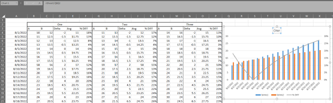
I have a bunch of data like is shown in the image. For each dataset (sets are titled "one", "two", "three"), I want to plot the values A, B, and % diff against the dates in column A. I don't want to keep manually editing the data selection for all 3 series each time I make a new graph, so I'm trying to understand how to write a macro to automate selecting the data depending on where on the sheet I've selected.

I'd like to be able to click in cell B2 or B3, run the macro, and have a chart pop up for dataset "one". The macro should know that $A$4:$A$21 is going to be my x-axis category for all series, regardless of dataset, but also know that because I clicked B2 (or B3, not sure if B2 being a merged cell would cause issues), I want B4:B21, C4:C21, and F4:F21 as my three series. The range will always be rows 4 to 21. Ideally, it'd also make the graph's title =B2. Likewise, if I clicked G2/3, it'd know that G, H, and K 4:21 are the three series.

Thank you!

 

[rlv01]

This might be something you can use the Macro Recorder for.

 

[ethaneandethaneproducts]

This might be something you can use the Macro Recorder for.

The trouble I'm having here is with the cell references - I know how to record a macro that'd make a chart for, say, B1:B10 on the y-axis and A1:A10 on the x-axis, but I'm not sure how I'd turn that into a macro that'd recognize that I'm in cell C1 and make a chart for C1:C10 on the y and A1:A10 on the x.

If I record myself making a chart from columns A, B, and C (with relative references enabled), it gives me

Sub Macro11()

'I started on "one", so I think this is saying go down 2, left 1 to find A4, select that, then select B1:C18
    ActiveCell.Offset(2, -1).Range("A1:A18,B1:C18").Select
'Not sure what this is 
    ActiveCell.Offset(2, 0).Range("A1").Activate
'adding the chart
    ActiveSheet.Shapes.AddChart2(201, xlColumnClustered).Select
'automatically setting the chart range 
    ActiveChart.SetSourceData Source:=Range("Sheet1!$A$4:$A$21,Sheet1!$B$4:$C$21" _
        )
        
End Sub

I'm not experienced with VBA (yet) but I'm not sure how I'd turn this into something that'd let me select the cell containing "one" "two" or "three", run the macro, and get the chart.

 

[ethaneandethaneproducts]

For clarity:

If I select range B2:F2 (labelled "one" in the picture I included), then run the macro I want A4:A21 (dates) as my category, and three series: B4:B21, C4:C21, F4:F21.

What I wish to be able to do is select G2:K2, then get G4:G21, H4:H21, and K4:K21 as series, with A4:A21 as category as usual.

Any ideas on how I could go about this? I'm stuck because recording macros always yields ranges, rather than "instructions" to select certain cells relative to the one I'm starting at.

 

[rlv01]

The trouble I'm having here is with the cell references - I know how to record a macro that'd make a chart for, say, B1:B10 on the y-axis and A1:A10 on the x-axis, but I'm not sure how I'd turn that into a macro that'd recognize that I'm in cell C1 and make a chart for C1:C10 on the y and A1:A10 on the x.

If I record myself making a chart from columns A, B, and C (with relative references enabled), it gives me

Sub Macro11()

'I started on "one", so I think this is saying go down 2, left 1 to find A4, select that, then select B1:C18
    ActiveCell.Offset(2, -1).Range("A1:A18,B1:C18").Select
'Not sure what this is
    ActiveCell.Offset(2, 0).Range("A1").Activate
'adding the chart
    ActiveSheet.Shapes.AddChart2(201, xlColumnClustered).Select
'automatically setting the chart range
    ActiveChart.SetSourceData Source:=Range("Sheet1!$A$4:$A$21,Sheet1!$B$4:$C$21" _
        )
       
End Sub

I'm not experienced with VBA (yet) but I'm not sure how I'd turn this into something that'd let me select the cell containing "one" "two" or "three", run the macro, and get the chart.

There are a couple of problems as I see it. One is that the code above is too 'clean' for the macro recorder. Two is that the chart image you posted is not a simple chart and your recorded macro does not reflect that. The point of the recorded macro is to understand the range syntax needed to create the chart you want. In your image, Series 1 & 2 are plotted as clustered bar charts, but series 3 is either an XY scatter plot or a line chart that resides on a secondary Y axis. Creating that would have been a specific manual action after the initial chart creation, and the macro recorder code would show that that but it does not.

Sub MakePlot()
    
    Dim PlotRange As Range
    Dim R As Range
    
    Select Case ActiveCell.Value
        Case "One", "Two", "Three"
        Case Else
            MsgBox "Invalid Selection" & vbCr & vbCr & "Please select valid chart data", vbCritical
            Exit Sub
    End Select
    
    Set R = ActiveCell
    Set PlotRange = Application.Union(R.EntireRow.Range("A1").Offset(1, 0).Resize(19, 1), R.Offset(1, 0).Resize(19, 2), R.Offset(1, 0).Offset(0, 4).Resize(19, 1))
    
    ActiveSheet.Shapes.AddChart2(201, xlColumnClustered).Select
    With ActiveChart
        .SetSourceData Source:=PlotRange
        .ChartTitle.Text = R.Text
        .FullSeriesCollection(3).AxisGroup = 2
        .FullSeriesCollection(3).ChartType = xlXYScatterLinesNoMarkers
    End With
End Sub

 

[ethaneandethaneproducts]

There are a couple of problems as I see it. One is that the code above is too 'clean' for the macro recorder. Two is that the chart image you posted is not a simple chart and your recorded macro does not reflect that. The point of the recorded macro is to understand the range syntax needed to create the chart you want. In your image, Series 1 & 2 are plotted as clustered bar charts, but series 3 is either an XY scatter plot or a line chart that resides on a secondary Y axis. Creating that would have been a specific manual action after the initial chart creation, and the macro recorder code would show that that but it does not.

Sub MakePlot()
   
    Dim PlotRange As Range
    Dim R As Range
   
    Select Case ActiveCell.Value
        Case "One", "Two", "Three"
        Case Else
            MsgBox "Invalid Selection" & vbCr & vbCr & "Please select valid chart data", vbCritical
            Exit Sub
    End Select
   
    Set R = ActiveCell
    Set PlotRange = Application.Union(R.EntireRow.Range("A1").Offset(1, 0).Resize(19, 1), R.Offset(1, 0).Resize(19, 2), R.Offset(1, 0).Offset(0, 4).Resize(19, 1))
   
    ActiveSheet.Shapes.AddChart2(201, xlColumnClustered).Select
    With ActiveChart
        .SetSourceData Source:=PlotRange
        .ChartTitle.Text = R.Text
        .FullSeriesCollection(3).AxisGroup = 2
        .FullSeriesCollection(3).ChartType = xlXYScatterLinesNoMarkers
    End With
End Sub

The trouble I'm having is specifically with the data selection portion of the code - I have 60 something cases like "one", "two", "three", but each is named for the data it represents. I'm mainly just trying to find an elegant way to avoid manually selecting the data for each and every plot I create. I'd neglected to include any chart formatting stuff in the macro because I figured it'd be easy to work out afterwards, but am now thinking that maybe making that third series (the % difference) a line may also pose a challenge.

 

[ethaneandethaneproducts]

There are a couple of problems as I see it. One is that the code above is too 'clean' for the macro recorder. Two is that the chart image you posted is not a simple chart and your recorded macro does not reflect that. The point of the recorded macro is to understand the range syntax needed to create the chart you want. In your image, Series 1 & 2 are plotted as clustered bar charts, but series 3 is either an XY scatter plot or a line chart that resides on a secondary Y axis. Creating that would have been a specific manual action after the initial chart creation, and the macro recorder code would show that that but it does not.

Sub MakePlot()
   
    Dim PlotRange As Range
    Dim R As Range
   
    Select Case ActiveCell.Value
        Case "One", "Two", "Three"
        Case Else
            MsgBox "Invalid Selection" & vbCr & vbCr & "Please select valid chart data", vbCritical
            Exit Sub
    End Select
   
    Set R = ActiveCell
    Set PlotRange = Application.Union(R.EntireRow.Range("A1").Offset(1, 0).Resize(19, 1), R.Offset(1, 0).Resize(19, 2), R.Offset(1, 0).Offset(0, 4).Resize(19, 1))
   
    ActiveSheet.Shapes.AddChart2(201, xlColumnClustered).Select
    With ActiveChart
        .SetSourceData Source:=PlotRange
        .ChartTitle.Text = R.Text
        .FullSeriesCollection(3).AxisGroup = 2
        .FullSeriesCollection(3).ChartType = xlXYScatterLinesNoMarkers
    End With
End Sub

Thank you though, this is almost exactly what I wanted. Is there a way to get around that

    Select Case ActiveCell.Value
        Case "One", "Two", "Three"
        Case Else
            MsgBox "Invalid Selection" & vbCr & vbCr & "Please select valid chart data", vbCritical
            Exit Sub
    End Select

chunk, and instead generalize it to any data formatted in this way?

 

[ethaneandethaneproducts]

Thank you though, this is almost exactly what I wanted. Is there a way to get around that

    Select Case ActiveCell.Value
        Case "One", "Two", "Three"
        Case Else
            MsgBox "Invalid Selection" & vbCr & vbCr & "Please select valid chart data", vbCritical
            Exit Sub
    End Select

chunk, and instead generalize it to any data formatted in this way?

Figured it out.

Sub MakePlot()
    
    Dim PlotRange As Range
    Dim R As Range
    
    Select Case ActiveCell.Value

    End Select
    
    Set R = ActiveCell
    Set PlotRange = Application.Union(R.EntireRow.Range("A1").Offset(1, 0).Resize(19, 1), R.Offset(1, 0).Resize(19, 2), R.Offset(1, 0).Offset(0, 4).Resize(19, 1))
    
    ActiveSheet.Shapes.AddChart2(201, xlColumnClustered).Select
    With ActiveChart
        .SetSourceData Source:=PlotRange
        .ChartTitle.Text = R.Text
        .FullSeriesCollection(3).AxisGroup = 2
        .FullSeriesCollection(3).ChartType = xlXYScatterLinesNoMarkers
    End With
End Sub

Just had to remove the stuff between Select Case and End Select