Macro to display highest value for a given range.

[Harishmz]

Hi team,

please could you help with a macro to solve the below problem?
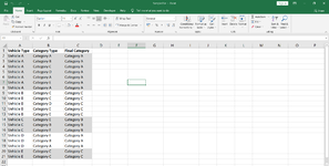
I have 2 columns - column 1 and column 2 with the below sample values. p1 is the highest value and p4 is the least value. Column 2 is a text column.
I want the highest value to be displayed in column 3 - "Output" based on column1.
For the range "Apples", the highest value is p1, orange it is p2 and grapes it is p4.

Column 1	Column 2	Output
Apples	p3	p1
Apples	p1	p1
Apples	p2	p1
Apples	p4	p1
Orange	p3	p2
Orange	p2	p2
Orange	p3	p2
Grapes	p4	p4

 

[Marc L]

Hi,​

​

unclear as here 'p1' is the lowest …​

 

[Harishmz]

Hi Marc,
just for representation purpose, I have considered p1 as the highest. It is like p1 is highest followed by p2, p3 and p4.

 

[Joe4]

just for representation purpose, I have considered p1 as the highest. It is like p1 is highest followed by p2, p3 and p4.

Do the values really look like "p1", "p2", etc, or are they really numeric?

To get the post possible help, it is advised to represent the data as it really exists. Don't try "simplify" things.
I have seen many instances where people do this, and they get an answer that works for their "simplified" example, but not for their actual data. So it doesn't really solve their problem.

 

[Marc L]

​

Attach at least a sample worksheet well respecting the Logic …​

 

[Harishmz]

Sure for the information. I will post with the correct values. Thanks.

 

[Harishmz]

I have attached a sample image.
Vehicle Type and Category Type are the available columns.
Category A is considered to be highest category followed by Category B, C, D and Category E. The highest category has to be displayed in 'Final Category Type' column.
Example,
for Vehicle B , the highest category is Category C and the value is displayed in column C.
Let me know if it makes sense.

 

[Joe4]

Is that really what your data looks like?
Then what determines the "highest" and "lowest" values?
Is it simply a matter of which comes first alphabetically?
If not, then you need to provide us with the logic for identifying highest/lowest (just explain it, in plain English).

 

[Marc L]

​

As I can do nothing with a picture … But obviously your highest is the lowest ! ​

 

[Joe4]

If it is really in alphabetic order, then one simple way would be to do the following:
1. Sort your data, primary sort on column A, secondary sort on column B, in ascending order.
2. Place this formula in cell C2 and copy down for all rows:

=IF(A2=A1,C1,B2)