etaf
Well-known Member
- Joined
- Oct 24, 2012
- Messages
- 8,276
- Office Version
- 365
- Platform
- MacOS
This is a nice to have at the moment
and i'm always interested in alternative ways to do things - BUT the main user of a larger spreadsheet i'm putting together is using 2016 , and may update later - BUT i would like if possible to male this work in 2016 version as well
For simplicity, I have created a very simple sample - just for the forum, which also works in the real data workbook, so hopefully no issues when i apply to the larger book
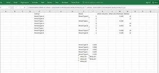
I have a formula in 365 version - using a UNQUE & FILTER function
This extracts a UNIQUE list , based on 2 NON-Contiguous columns , column A will contain blanks , which need to be ignored, as there will be a thickness and i dont want a group BLANK/THICKNESS
This is part of a much bigger spreadsheet and so I do NOT want to incorporate a pivot table as its part of a larger table , although i would use a pivot table if no simple solution, and change the layout - I have the pivot table in my example - XL2BB has shown the pivot table - BUT i have also put the sample on a share dropbox
I also do not want VBA - as again its part of a larger spreadsheet and avoiding VBA as much as possible, if i do add VBA later then i can incorporate it , but the vision is not to at the moment
Not end of world if not easy with Older 2016 versions Functions to replicate , its just the main person using the spreadsheet currently has 2016 version, although may in the future upgrade.... and i see a similar possible spreadsheet for my daughter framing material - and she has 2016 Mac version i think (which maybe 2011)
Sort is not that important - just i can do it in 365
=SORT(UNIQUE(FILTER(FILTER(A2:D9,A2:A9<>""),{1,0,0,1})))
I know the {1,0,0,1} allow for the NON Contiguous ranges - so only the 2 columns are output - WOOD/THICKNESS
And i found the Filter(Filter ( Excel Filter Function Trick Using Non-Adjacent Columns - Xelplus - Leila Gharani ) - part to also be able to add a criteria so blanks are ignored - which will appear anywhere in rows - and again the main table cannot be sorted
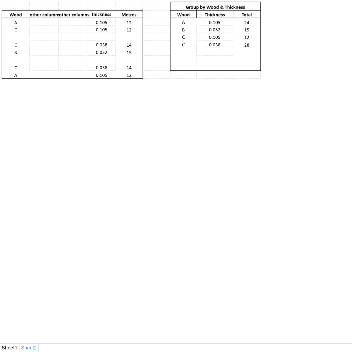
Then once i have extracted the UNIQUE Wood Type and Thickness - i then use a simple SUMIFS() to group into material - which is what i'm after
Thanks for looking
and i'm always interested in alternative ways to do things - BUT the main user of a larger spreadsheet i'm putting together is using 2016 , and may update later - BUT i would like if possible to male this work in 2016 version as well
For simplicity, I have created a very simple sample - just for the forum, which also works in the real data workbook, so hopefully no issues when i apply to the larger book
I have a formula in 365 version - using a UNQUE & FILTER function
This extracts a UNIQUE list , based on 2 NON-Contiguous columns , column A will contain blanks , which need to be ignored, as there will be a thickness and i dont want a group BLANK/THICKNESS
This is part of a much bigger spreadsheet and so I do NOT want to incorporate a pivot table as its part of a larger table , although i would use a pivot table if no simple solution, and change the layout - I have the pivot table in my example - XL2BB has shown the pivot table - BUT i have also put the sample on a share dropbox
I also do not want VBA - as again its part of a larger spreadsheet and avoiding VBA as much as possible, if i do add VBA later then i can incorporate it , but the vision is not to at the moment
Not end of world if not easy with Older 2016 versions Functions to replicate , its just the main person using the spreadsheet currently has 2016 version, although may in the future upgrade.... and i see a similar possible spreadsheet for my daughter framing material - and she has 2016 Mac version i think (which maybe 2011)
Sort is not that important - just i can do it in 365
=SORT(UNIQUE(FILTER(FILTER(A2:D9,A2:A9<>""),{1,0,0,1})))
I know the {1,0,0,1} allow for the NON Contiguous ranges - so only the 2 columns are output - WOOD/THICKNESS
And i found the Filter(Filter ( Excel Filter Function Trick Using Non-Adjacent Columns - Xelplus - Leila Gharani ) - part to also be able to add a criteria so blanks are ignored - which will appear anywhere in rows - and again the main table cannot be sorted
Then once i have extracted the UNIQUE Wood Type and Thickness - i then use a simple SUMIFS() to group into material - which is what i'm after
| Group-Summary.xlsx | ||||||||||||||||
|---|---|---|---|---|---|---|---|---|---|---|---|---|---|---|---|---|
| A | B | C | D | E | F | G | H | I | J | K | L | M | N | |||
| 1 | Wood | other columns | other columns | thickness | Metres | Group by Wood & Thickness | ||||||||||
| 2 | A | 0.105 | 12 | Wood | Thickness | Total | Wood | thickness | Sum of Metres | |||||||
| 3 | C | 0.105 | 12 | A | 0.105 | 24 | A | 0.105 | 24 | |||||||
| 4 | B | 0.052 | 15 | B | 0.052 | 15 | ||||||||||
| 5 | C | 0.038 | 14 | C | 0.105 | 12 | C | 0.105 | 12 | |||||||
| 6 | B | 0.052 | 15 | C | 0.038 | 28 | 0.038 | 28 | ||||||||
| 7 | ||||||||||||||||
| 8 | C | 0.038 | 14 | |||||||||||||
| 9 | A | 0.105 | 12 | |||||||||||||
Sheet1 | ||||||||||||||||
| Cell Formulas | ||
|---|---|---|
| Range | Formula | |
| G3:H6 | G3 | =SORT(UNIQUE(FILTER(FILTER(A2:D9,A2:A9<>""),{1,0,0,1}))) |
| I3:I9 | I3 | =IF(G3="","",SUMIFS($E$2:$E$9,$A$2:$A$9,G3,$D$2:$D$9,H3)) |
| Dynamic array formulas. | ||
Thanks for looking