Making a list of duplicates by searching 6 columns and using 2 criteria

[Zacariah171]

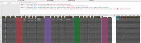
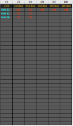
I have been able to make a list in column CY that lists any duplicates found in columns D, J, P, and V. Any duplicates found in those columns are listed once in CY. I have the formula written for that listed below and it works fine. Now, I'd like to alter that formula so that it will just list any duplicates that have "PRI" in the column next to it: E, K, Q, and W. I just cant seem to figure out how to add in that extra criteria. In the attached picture, the only item that should be listed in column CY should be Unit 56. Unit 11 is listed twice in column D but only one of those has a Status of PRI next to it, so it's not a duplicate that I'm looking for and should not be listed in CY. Unit 56 is listed twice; once in column D and once in column J and both have a Status of PRI, so that is a duplicate that I'm looking for, so it should be listed once in CY7. Any help is greatly appreciated and please let me know if you need more information.

This is the formula I'm looking to alter to accommodate the extra criteria.
=IFNA(IFERROR(IFERROR(IFERROR(
LOOKUP(2, 1/((COUNTIF($CY$6:CY6, $D$7:$D$37)=0)*(COUNTIF($D$7:$D$37, $D$7:$D$37)>1)), $D$7:$D$37),
LOOKUP(2, 1/((COUNTIF($CY$6:CY6, $J$7:$J$37)=0)*((COUNTIF($J$7:$J$37, $J$7:$J$37)>1)+(COUNTIF($D$7:$D$37, $J$7:$J$37)>0))),$J$7:$J$37)),
LOOKUP(2, 1/((COUNTIF($CY$6:CY6, $P$7:$P$37)=0)*((COUNTIF($P$7:$P$37, $P$7:$P$37)>1)+(COUNTIF($D$7:$D$37, $P$7:$P$37)>0)+(COUNTIF($J$7:$J$37, $P$7:$P$37)>0))), $P$7:$P$37)),
LOOKUP(2, 1/((COUNTIF($CY$6:CY6, $V$7:$V$37)=0)*((COUNTIF($V$7:$V$37, $V$7:$V$37)>1)+(COUNTIF($D$7:$D$37, $V$7:$V$37)>0)+(COUNTIF($J$7:$J$37, $V$7:$V$37)>0)+(COUNTIF($P$7:$P$37, $V$7:$V$37)>0))), $V$7:$V$37)), "")

Thank you.

 

[maabadi]

Please upload your example file & Desired Results with XL2BB ADDIN (Preferable) OR upload it at free uploading site e.g. www.dropbox.com or googledrive or onedrive and insert link here.

 

[Zacariah171]

Thanks for the reply. Ok. First time uploading a mini-sheet. Please let me know if there's anything else you need with it. In the example on the sheet, Unit 11 is listed twice in column D but it's not a duplicate that I'm looking for because only one of them has the Status "PRI", so it should not be showing up in my list in the CY column. Unit 56 is listed twice, once in column D and once in column J, and both have the Status "PRI", so that Unit 56 should show up in my CY column. In the CZ column next to it, "1st Box" should be 75 (From column A), and DA "2nd Box" should be 71 (From column A). Unit 22 is listed across the table 5 times but only 3 have the "PRI" Status, so it should be listed in CY and in column CZ next to in the "1st Box" should be 101, "2nd Box" should be 101, and "3rd Box" should be 108. I hope that provides enough detail of what I'm trying to accomplish.

Datalog Monthly Usage_11.xlsm
	A	B	C	D	E	F	G	H	I	J	K	L	M	N	O	P	Q	R	S	T	U	V	W
6	ID	Received	Returned	Unit 1	Status 1	Start 1	End 1	Days 1	Location 1	Unit 2	Status 2	Start 2	End 2	Days 2	Location 2	Unit 3	Status 3	Start 3	End 3	Days 3	Location 3	Unit 4	Status 4
7	074			Unit 11	PRI	1/3	1/23	21	Oklahoma
8	071			Unit 11	BU				Oklahoma	Unit 56	PRI	1/22	1/28	7	Oklahoma
9	075			Unit 56	PRI	1/4	1/21	18	Oklahoma
10	101			Unit 22	PRI	1/2	1/15	14	Texas	Unit 22	PRI	1/18	1/23	6	Texas
11	106			Unit 22	BU				Texas	Unit 22	BU				Texas
12	108															Unit 22	PRI	1/24	1/31	8
13	136
14	138
15	151
16	159
17	185
18	189
19	190
20	301
21	302
22	307
23	385
24	481
25	802
26	839
27	811
28	814
29	816
30	818
31	824
32	830
33	832
34	833
35	838
36	854
37	856
Jan 2021

Cell Formulas
Range	Formula
H7:H37	H7	=IF(AND([@[Start 1]]<>"", [@[End 1]]<>""), DAYS([@[End 1]],[@[Start 1]])+1, 0)
N7:N37	N7	=IF(AND([@[Start 2]]<>"", [@[End 2]]<>""), DAYS([@[End 2]],[@[Start 2]])+1, 0)
T7:T37	T7	=IF(AND([@[Start 3]]<>"", [@[End 3]]<>""), DAYS([@[End 3]],[@[Start 3]])+1, 0)

Cells with Conditional Formatting
Cell	Condition		Cell Format	Stop If True
H36,Z36,T36,N36	Cell Value	=0	text	NO
H35,Z35,T35,N35	Cell Value	=0	text	NO
H34,Z34,T34,N34	Cell Value	=0	text	NO
H33,Z33,T33,N33	Cell Value	=0	text	NO
H32,Z32,T32,N32	Cell Value	=0	text	NO
H31,Z31,T31,N31	Cell Value	=0	text	NO
H37:H39,Z37:Z39,T37:T39,N37:N39,N41:N1048576,T41:T1048576,Z41:Z1048576,H41:H1048576	Cell Value	=0	text	NO

Cells with Data Validation
Cell	Allow	Criteria
D7:D37	List	='Data Validation Table'!$A$3:$A$102
E7:E37	List	='Data Validation Table'!$C$3:$C$5
I7:I37	List	='Data Validation Table'!$B$3:$B$11
J7:J37	List	='Data Validation Table'!$A$3:$A$102
K7:K37	List	='Data Validation Table'!$C$3:$C$5
O7:O37	List	='Data Validation Table'!$B$3:$B$11
P7:P37	List	='Data Validation Table'!$A$3:$A$102
Q7:Q37	List	='Data Validation Table'!$C$3:$C$5
U7:U37	List	='Data Validation Table'!$B$3:$B$11
V7:V37	List	='Data Validation Table'!$A$3:$A$102
W7:W37	List	='Data Validation Table'!$C$3:$C$5

 

[Zacariah171]

I couldn't load everything I needed to in the first mini-sheet and when I try to load another mini **** for the rest, which isn't too much, I get a message saying that I've exceeded my limit. So, here is a screenshot of the results table and a sample of the formulas used. I hope this helps.

Formula in CY7:
=IFNA(IFERROR(IFERROR(IFERROR(
LOOKUP(2, 1/((COUNTIF($CY$6:CY6, $D$7:$D$37)=0)*(COUNTIF($D$7:$D$37, $D$7:$D$37)>1)), $D$7:$D$37),
LOOKUP(2, 1/((COUNTIF($CY$6:CY6, $J$7:$J$37)=0)*((COUNTIF($J$7:$J$37, $J$7:$J$37)>1)+(COUNTIF($D$7:$D$37, $J$7:$J$37)>0))),$J$7:$J$37)),
LOOKUP(2, 1/((COUNTIF($CY$6:CY6, $P$7:$P$37)=0)*((COUNTIF($P$7:$P$37, $P$7:$P$37)>1)+(COUNTIF($D$7:$D$37, $P$7:$P$37)>0)+(COUNTIF($J$7:$J$37, $P$7:$P$37)>0))), $P$7:$P$37)),
LOOKUP(2, 1/((COUNTIF($CY$6:CY6, $V$7:$V$37)=0)*((COUNTIF($V$7:$V$37, $V$7:$V$37)>1)+(COUNTIF($D$7:$D$37, $V$7:$V$37)>0)+(COUNTIF($J$7:$J$37, $V$7:$V$37)>0)+(COUNTIF($P$7:$P$37, $V$7:$V$37)>0))), $V$7:$V$37)), "")

Formula in CZ7
=IF($CY7="", "", IFERROR(INDEX($A$7:$A$37,SMALL(IF($D$7:$D$37:$J$7:$J$37:$P$7:$P$37:$V$7:$V$37=$CY7,ROW($A$7:$A$37)-MIN(ROW($A$7:$A$37))+1),COLUMNS($CY7:CY7))),""))

Formula in DA7
=IF($CY7="", "", IFERROR(INDEX($A$7:$A$37,SMALL(IF($D$7:$D$37:$J$7:$J$37:$P$7:$P$37:$V$7:$V$37=$CY7,ROW($A$7:$A$37)-MIN(ROW($A$7:$A$37))+1),COLUMNS($CY7:CZ7))),""))

 

[maabadi]

I understand What exactly You want, But with your Table Structure , it is very Hard & long Formula.
You Should Change Your Table Structure To this to Search Units At One Column & Status At One Column.

This is Example:

TEST.xlsx
	A	B	C	D	E	F	G	H	I	J	K	L	M	N	O	P	Q	R	S	T
1	ID	Received	Returned	Unit	Unit Type	Status	Start	End	Days	Location		Countifs		Unit	Status	1	2	3	4
2	74			Unit 11	1	PRI	44199	44219	21	Oklahoma		1		Unit 56	PRI	75	71
3	71			Unit 11	1	BU			0	Oklahoma		1		Unit 22	PRI	101	101	108
4	75			Unit 56	1	PRI	44200	44217	18	Oklahoma		1		Unit 22	BU	106	106
5	101			Unit 22	1	PRI	44198	44211	14	Texas		1
6	106			Unit 22	1	BU			0	Texas		1
7	74				2				0			0
8	71			Unit 56	2	PRI	44218	44224	7	Oklahoma		2
9	75				2				0			0
10	101			Unit 22	2	PRI	44214	44219	6	Texas		2
11	106			Unit 22	2	BU			0	Texas		2
12	74				3				0			0
13	71				3				0			0
14	75				3				0			0
15	101				3				0			0
16	106				3				0			0
17	108			Unit 22	3	PRI	44220	44227	8			3
18
Sheet2

Cell Formulas
Range	Formula
N2:N17	N2	=IFERROR(INDEX(Table2[Unit],SMALL(IF(($L$2:$L$17=2), ROW(Table2[Unit])-ROW($D$2)+1),ROWS($N$1:N1))),"")
O2:O17	O2	=IFERROR(INDEX(Table2[Status],SMALL(IF(($L$2:$L$17=2), ROW(Table2[Status])-ROW($F$2)+1),ROWS($O$1:O1))),"")
P2:S17	P2	=IFERROR(IF(N2="","",INDEX(Table2[ID],SMALL(IF((Table2[Unit]=$N2)*(Table2[Status]=$O2), ROW(Table2[Days])-ROW($I$2)+1),COLUMNS($P$1:P1)))),"")
I2:I17	I2	=IF(AND([@Start]<>"", [@End]<>""), DAYS([@End],[@Start])+1, 0)
L2:L17	L2	=COUNTIFS($D$2:D2,D2,$F$2:F2,F2)
Press CTRL+SHIFT+ENTER to enter array formulas.

 

[Zacariah171]

Unfortunately, restructuring the table like that wont work because it would change way too many other things in my sheet. Thank you for your time looking into it though.

 

[maabadi]

What about Create New Table Structure at new Sheet with macro (VBA)?
And then Do calculation on it and finally Paste Results at range you want ( we can do all of this with Macro)

 

[maabadi]

If its OK, I add Transported Data At Sheet2 and then Extract what you want and Paste Back at Sheet1

Option Explicit

Sub TransformData2()
Dim i As Long, j As Long, Sh1 As Worksheet, Sh2 As Worksheet, Lr As Long, Lr1 As Long, Lr2 As Long
Dim K As Long, L As Long, M As Long, N As Long, P As Long, Lr3 As Long
Set Sh1 = Sheets("Sheet1")
Set Sh2 = Sheets("Sheet2")
Lr = Sh1.Cells(Rows.Count, 1).End(xlUp).Row
For i = Lr To 7 Step -1
If Sh1.Cells(i, 4).Value <> "" Then
K = i
GoTo Res2
End If
Next i
Res2:
Lr1 = 7
Lr2 = K
Sh2.Range("A6:C6").Value = Sh1.Range("A6:C6").Value
For j = 4 To 9
Sh2.Cells(6, j).Value = Left(Sh1.Cells(6, j).Value, Len(Sh1.Cells(6, j).Value) - 1)
Next j
Sh2.Range("J6").Value = "Unit Type"
Sh2.Range("K6").Value = "CountIFS"
For j = 4 To 26 Step 6
For i = 7 To K
If Sh1.Cells(i, j).Value <> "" Then
M = Lr2 - (Lr1 + K) + i + 7
N = Lr1 + i - (7 + P)
Sh2.Range("A" & N & ":C" & N).Value = Sh1.Range("A" & M & ":C" & M).Value
Range(Sh1.Cells(M, j), Sh1.Cells(M, j + 5)).Copy Sh2.Cells(N, 4)
Sh2.Range("J" & N).Value = "Unit" & (Int(j / 6) + 1)
Sh2.Range("K" & N).Value = Application.WorksheetFunction.CountIfs(Sh2.Range("D2:D" & N), Sh2.Range("D" & N), Sh2.Range("E2:E" & N), Sh2.Range("E" & N))
Else
P = P + 1
End If
Next i
For i = Lr To 2 Step -1
If Sh1.Cells(i, j + 6).Value <> "" Then
K = i
GoTo Res3
End If
Next i
Res3:
Lr1 = Lr2 + 1
Lr2 = Lr2 + K - 6
Next j

With Sh2
Lr2 = .Cells(Rows.Count, 11).End(xlUp).Row
P = 7
.Range("M6").Value = "Unit"
.Range("N6").Value = "Status"
For i = 7 To Lr2
If Sh2.Cells(i, 11).Value = 2 Then
.Range("M" & P).Value = .Range("D" & i).Value
.Range("N" & P).Value = .Range("E" & i).Value
P = P + 1
End If
Next i
Lr3 = .Cells(Rows.Count, 11).End(xlUp).Row
For j = 15 To 19
Sh2.Cells(6, j).Value = j - 14
Next j

For i = 7 To Lr3
j = 15
For L = 7 To Lr2
If .Range("M" & i).Value = .Range("D" & L).Value And .Range("N" & i).Value = .Range("E" & L).Value Then
.Cells(i, j).Value = .Range("A" & L).Value
j = j + 1
End If
Next L
Next i
End With
Sh2.Range("M6:S" & Lr3).Copy Sh1.Range("CY6:DD" & Lr3)

End Sub

 

[Zacariah171]

Thank you for your time you spent working on this. I went a different route and it seems to be working ok. I wound up just making a 5 helper columns, DF7:DJ37. The first column was just a copy of column A. The 2nd helper was just a simple index match formula that looked at column E for "PRI" and returned the value in column D. The 3rd helper column did the same thing with columns J and K, the 4th helper column for columns P and Q, and the 5th helper for columns V and W. So this basically makes the same table as the original but without all the extra columns and it only displays the Units that had PRI next to them in the original table.

Utilization.xlsm
	DF	DG	DH	DI	DJ	DK
3
4	Only list the "Primary" Units/Equipment
6		Unit 1	Unit 2	Unit 3	Unit 4
7	074	Unit 11
8	071		Unit 56
9	075	Unit 56
10	101	Unit 22	Unit 22
11	106
12	108			Unit 22
13	136
14	138
15	151
16	159
17	185
18	189
19	190
20	301
21	302
22	307
23	385
24	481
25	802
26	839
27	811
28	814
29	816
30	818
31	824
32	830
33	832
34	833
35	838
36	854
37	856
38	000
39
Jan 2021

Cell Formulas
Range	Formula
DF7:DF38	DF7	=A7
DG7:DG38	DG7	=IFNA(INDEX($D7, MATCH('Data Validation Table'!$C$3, $E7, 0)), "")
DH7:DH38	DH7	=IFNA(INDEX($J7, MATCH('Data Validation Table'!$C$3, $K7, 0)), "")
DI7:DI38	DI7	=IFNA(INDEX($P7, MATCH('Data Validation Table'!$C$3, $Q7, 0)), "")
DJ7:DJ38	DJ7	=IFNA(INDEX($V7, MATCH('Data Validation Table'!$C$3, $W7, 0)), "")

Next, I recreated the same table that was in my second post (the one that listed the 1st, 2nd, 3, 4, and 5th boxes) and put it in DM7:DR37. The formula I used in DM to search through DF7:DJ37 and list only the values that were listed more than once was

=IFNA(IFERROR(IFERROR(IFERROR(
LOOKUP(2, 1/((COUNTIF($DM$6:DM6, $DG$7:$DG$38)=0)*(COUNTIF($DG$7:$DG$38, $DG$7:$DG$38)>1)), $DG$7:$DG$38),
LOOKUP(2, 1/((COUNTIF($DM$6:DM6, $DH$7:$DH$38)=0)*((COUNTIF($DH$7:$DH$38, $DH$7:$DH$38)>1)+(COUNTIF($DG$7:$DG$38, $DH$7:$DH$38)>0))),$DH$7:$DH$38)),
LOOKUP(2, 1/((COUNTIF($DM$6:DM6, $DI$7:$DI$38)=0)*((COUNTIF($DI$7:$DI$38, $DI$7:$DI$38)>1)+(COUNTIF($DG$7:$DG$38, $DI$7:$DI$38)>0)+(COUNTIF($DH$7:$DH$38, $DI$7:$DI$38)>0))), $DI$7:$DI$38)),
LOOKUP(2, 1/((COUNTIF($DM$6:DM6, $DJ$7:$DJ$38)=0)*((COUNTIF($DJ$7:$DJ$38, $DJ$7:$DJ$38)>1)+(COUNTIF($DG$7:$DG$38, $DJ$7:$DJ$38)>0)+(COUNTIF($DH$7:$DH$38, $DJ$7:$DJ$38)>0)+(COUNTIF($DI$7:$DI$38, $DJ$7:$DJ$38)>0))), $DJ$7:$DJ$38)), "")

Then, the formula I used in columns DN:DR to list the boxes associated was

=IF($DM7="", "", IFERROR(INDEX($DF$7:$DF$38,SMALL(IF($DG$7:$DJ$38=$DM7,ROW($DF$7:$DF$38)-MIN(ROW($DF$7:$DF$38))+1),COLUMNS($DM7:DM7))),""))

Utilization.xlsm
	DM	DN	DO	DP	DQ	DR
3
4	Only list the Equip that was marked as PRI for each Unit
6		1st Box	2nd Box	3rd Box	4th Box	5th Box
7	Unit 22	101	101	108
8	Unit 56	71	75
9
10
11
12
13
14
15
16
17
18
19
20
21
22
23
24
25
26
27
28
29
30
31
32
33
34
35
36
37
38
39
Jan 2021

Cell Formulas
Range	Formula
DM7:DM36	DM7	=IFNA(IFERROR(IFERROR(IFERROR( LOOKUP(2, 1/((COUNTIF($DM$6:DM6, $DG$7:$DG$38)=0)*(COUNTIF($DG$7:$DG$38, $DG$7:$DG$38)>1)), $DG$7:$DG$38), LOOKUP(2, 1/((COUNTIF($DM$6:DM6, $DH$7:$DH$38)=0)*((COUNTIF($DH$7:$DH$38, $DH$7:$DH$38)>1)+(COUNTIF($DG$7:$DG$38, $DH$7:$DH$38)>0))),$DH$7:$DH$38)), LOOKUP(2, 1/((COUNTIF($DM$6:DM6, $DI$7:$DI$38)=0)*((COUNTIF($DI$7:$DI$38, $DI$7:$DI$38)>1)+(COUNTIF($DG$7:$DG$38, $DI$7:$DI$38)>0)+(COUNTIF($DH$7:$DH$38, $DI$7:$DI$38)>0))), $DI$7:$DI$38)), LOOKUP(2, 1/((COUNTIF($DM$6:DM6, $DJ$7:$DJ$38)=0)*((COUNTIF($DJ$7:$DJ$38, $DJ$7:$DJ$38)>1)+(COUNTIF($DG$7:$DG$38, $DJ$7:$DJ$38)>0)+(COUNTIF($DH$7:$DH$38, $DJ$7:$DJ$38)>0)+(COUNTIF($DI$7:$DI$38, $DJ$7:$DJ$38)>0))), $DJ$7:$DJ$38)), "")
DN7:DR38	DN7	=IF($DM7="", "", IFERROR(INDEX($DF$7:$DF$38,SMALL(IF($DG$7:$DJ$38=$DM7,ROW($DF$7:$DF$38)-MIN(ROW($DF$7:$DF$38))+1),COLUMNS($DM7:DM7))),""))
DM37:DM38	DM37	=IFNA(IFERROR(IFERROR(IFERROR( LOOKUP(2, 1/((COUNTIF($DM$6:DM35, $DG$7:$DG$38)=0)*(COUNTIF($DG$7:$DG$38, $DG$7:$DG$38)>1)), $DG$7:$DG$38), LOOKUP(2, 1/((COUNTIF($DM$6:DM35, $DH$7:$DH$38)=0)*((COUNTIF($DH$7:$DH$38, $DH$7:$DH$38)>1)+(COUNTIF($DG$7:$DG$38, $DH$7:$DH$38)>0))),$DH$7:$DH$38)), LOOKUP(2, 1/((COUNTIF($DM$6:DM35, $DI$7:$DI$38)=0)*((COUNTIF($DI$7:$DI$38, $DI$7:$DI$38)>1)+(COUNTIF($DG$7:$DG$38, $DI$7:$DI$38)>0)+(COUNTIF($DH$7:$DH$38, $DI$7:$DI$38)>0))), $DI$7:$DI$38)), LOOKUP(2, 1/((COUNTIF($DM$6:DM35, $DJ$7:$DJ$38)=0)*((COUNTIF($DJ$7:$DJ$38, $DJ$7:$DJ$38)>1)+(COUNTIF($DG$7:$DG$38, $DJ$7:$DJ$38)>0)+(COUNTIF($DH$7:$DH$38, $DJ$7:$DJ$38)>0)+(COUNTIF($DI$7:$DI$38, $DJ$7:$DJ$38)>0))), $DJ$7:$DJ$38)), "")

 

[maabadi]

Glad You can Do it. Good Luck.