Match a value but return a different column value without duplicates

[aheffy]

I'm working with a large amount of data in two separate tabs:

Tab X: Column A (Product #) contains a list of product numbers (e.g. 700, 701, etc). Column B (Load ID) contains a unique ID for one specific unit of that product (e.g. 12345, 12346, etc).

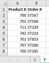
Tab Y: Column A (Product #) contains a list of product numbers again (e.g. 700, 701, etc). Column B (Order #) contains a list of customer orders (e.g. ST567, ST568).

I am trying to match the product numbers in tab X with the product numbers in tab Y and return a unique customer order number (column B) that relates to that product number. However, I can only use each order number once, I can't have duplicates. Put differently, I am attempting to pair unique ID's of various product numbers to unique order numbers of the same product without duplicates.

I've attempted various index and match formulae as well as various vlookup formulae with nested ifs. I don't believe I have gotten close with either of these.

Thank you in advance for any help you can provide!!!

 

[strooman]

Can you provide a sample or screenshot with the desired result? We have to see how the layout of the data is.

 

[aheffy]

Sure! Sorry, I should I have done that from the beginning.

Can you provide a sample or screenshot with the desired result? We have to see how the layout of the data is.

 

[aheffy]

[/IMG]

 

[strooman]

OK, I presume that the image is from Tab X and that the yellow area is where the formula is inserted. Is this a correct assumption?

When this is a Yes, where do we lookup the Order # in column C? I mean, are the Order # in a table on Tab Y? If Yes then please send screenshot from Tab Y.

 

[aheffy]

OK, I presume that the image is from Tab X and that the yellow area is where the formula is inserted. Is this a correct assumption?

When this is a Yes, where do we lookup the Order # in column C? I mean, are the Order # in a table on Tab Y? If Yes then please send screenshot from Tab Y.

Yes, your assumption is correct. The yellow area is where the formula will be inserted on Tab X.

Here is a screenshot of Tab Y:

Thank you for your help!

 

[strooman]

Well, it's a difficult lookup because you got nothing to go on. You only have the Product# and there are duplicates as you mentioned.
The only thing I can think of is to insert a helper column in COLUMN E.

Formula's:

In C2:

=IFERROR(VLOOKUP($A2&"-"&COUNTIF($A$2:$A2;$A2);$E$2:$G$25;3;FALSE);"")

And copy down.

In E2 (the helper column):

=$F2&"-"&COUNTIF($F$2:F2;F2)

And copy down.

Row\Col	A​	B​	C​	D​	E​	F​	G​
1​	Product_Number	Load_ID	Order_Number		Helper	Product_Number	Order_Number
2​	703​	12345​	ST361		709-1	709​	ST567
3​	708​	12346​			705-1	705​	ST568
4​	709​	12347​	ST567		701-1	701​	ST329
5​	701​	12348​	ST329		710-1	710​	ST210
6​	701​	12349​	ST853		701-2	701​	ST853
7​	702​	12350​	ST490		701-3	701​	ST580
8​	708​	12351​			707-1	707​	ST385
9​	700​	12352​	ST456		702-1	702​	ST490
10​	702​	12353​	ST381		704-1	704​	ST399
11​	704​	12354​	ST399		704-2	704​	ST443
12​	700​	12355​			705-2	705​	ST274
13​	705​	12356​	ST568		707-2	707​	ST494
14​	710​	12357​	ST210		707-3	707​	ST482
15​	705​	12358​	ST274		710-2	710​	ST242
16​	703​	12359​	ST407		710-3	710​	ST416
17​	700​	12360​			709-2	709​	ST275
18​	710​	12361​	ST242		704-3	704​	ST317
19​	703​	12362​			709-3	709​	ST240
20​	703​	12363​			703-1	703​	ST361
21​	707​	12364​	ST385		710-4	710​	ST413
22​	710​	12365​	ST416		707-4	707​	ST486
23​	700​	12366​			702-2	702​	ST381
24​	707​	12367​	ST494		703-2	703​	ST407
25​	709​	12368​	ST275		700-1	700​	ST456
26​
27​	Tab X					Tab Y

You have to adjust the formula's so that they refere to your sheetnames.

 

[aheffy]

Well, it's a difficult lookup because you got nothing to go on. You only have the Product# and there are duplicates as you mentioned.
The only thing I can think of is to insert a helper column in COLUMN E.

Formula's:

In C2:

=IFERROR(VLOOKUP($A2&"-"&COUNTIF($A$2:$A2;$A2);$E$2:$G$25;3;FALSE);"")

And copy down.

In E2 (the helper column):

=$F2&"-"&COUNTIF($F$2:F2;F2)

And copy down.

Row\Col	A​	B​	C​	D​	E​	F​	G​
1​	Product_Number	Load_ID	Order_Number		Helper	Product_Number	Order_Number
2​	703​	12345​	ST361		709-1	709​	ST567
3​	708​	12346​			705-1	705​	ST568
4​	709​	12347​	ST567		701-1	701​	ST329
5​	701​	12348​	ST329		710-1	710​	ST210
6​	701​	12349​	ST853		701-2	701​	ST853
7​	702​	12350​	ST490		701-3	701​	ST580
8​	708​	12351​			707-1	707​	ST385
9​	700​	12352​	ST456		702-1	702​	ST490
10​	702​	12353​	ST381		704-1	704​	ST399
11​	704​	12354​	ST399		704-2	704​	ST443
12​	700​	12355​			705-2	705​	ST274
13​	705​	12356​	ST568		707-2	707​	ST494
14​	710​	12357​	ST210		707-3	707​	ST482
15​	705​	12358​	ST274		710-2	710​	ST242
16​	703​	12359​	ST407		710-3	710​	ST416
17​	700​	12360​			709-2	709​	ST275
18​	710​	12361​	ST242		704-3	704​	ST317
19​	703​	12362​			709-3	709​	ST240
20​	703​	12363​			703-1	703​	ST361
21​	707​	12364​	ST385		710-4	710​	ST413
22​	710​	12365​	ST416		707-4	707​	ST486
23​	700​	12366​			702-2	702​	ST381
24​	707​	12367​	ST494		703-2	703​	ST407
25​	709​	12368​	ST275		700-1	700​	ST456
26​
27​	Tab X					Tab Y

<tbody>
</tbody>

You have to adjust the formula's so that they refere to your sheetnames.

That did it! Thank you so much for your help. I should have thought of that, but I didn't and I don't think it was going to come to me overnight. Much appreciated!

 

[strooman]

Thanks for the feedback. Glad i could help.