Mad4xcel
New Member
- Joined
- Mar 26, 2022
- Messages
- 5
- Office Version
- 365
- 2021
- 2019
- 2016
- 2013
- Platform
- Windows
- MacOS
- Mobile
- Web
Hi All,
I have a three sheets, Sheet 1, Sheet 2, Sheet 3.
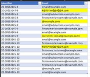
Sheet 1 has Id's and email addresses columns, Each Id has many emails, sometimes blanks too,. Each Id has multiple rows in Sheet 1.
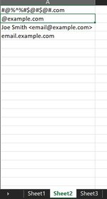
Sheet 2 has list of keywords words to use as exclude lists for email addresses.
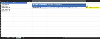
Sheet 3 has Id's, and Email addresses columns. Each Id is a unique row in Sheet 3.
I need to match Id's in sheet 3 to Id's in Sheet 1, get a list of unique, non blanks email addresses from sheet 1, filter out email addresses based on the sheet 2 exclude list keywords(partial matches), and concatenate all the emails (that are not partially matching the exclude list) with a concatenation operation like semi colon or comma.
I am not that good with array formula. I need to work on it, and many other things in excel.
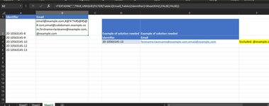
This rudimentary formula I have constructed identifies the ID from sheet 3 to all rows with the same ID in Sheet 1, gets the email addresses and concatenates them with a comma operator
I have not been able to progress on it despite many hours of trial and error. I would appreciate any help I can receive on it.
Thank you, everyone !
I have a three sheets, Sheet 1, Sheet 2, Sheet 3.
Sheet 1 has Id's and email addresses columns, Each Id has many emails, sometimes blanks too,. Each Id has multiple rows in Sheet 1.
Sheet 2 has list of keywords words to use as exclude lists for email addresses.
Sheet 3 has Id's, and Email addresses columns. Each Id is a unique row in Sheet 3.
I need to match Id's in sheet 3 to Id's in Sheet 1, get a list of unique, non blanks email addresses from sheet 1, filter out email addresses based on the sheet 2 exclude list keywords(partial matches), and concatenate all the emails (that are not partially matching the exclude list) with a concatenation operation like semi colon or comma.
I am not that good with array formula. I need to work on it, and many other things in excel.
This rudimentary formula I have constructed identifies the ID from sheet 3 to all rows with the same ID in Sheet 1, gets the email addresses and concatenates them with a comma operator
=TEXTJOIN(",",TRUE,UNIQUE(FILTER(Table1[Email],Table1[Identifier]=Sheet3!A2),FALSE,FALSE))I have not been able to progress on it despite many hours of trial and error. I would appreciate any help I can receive on it.
Thank you, everyone !