Hi there,
I'm working on a self-scheduling sheet for a group of 30 employees and I'm trying to figure out how to match two criteria and it populate a single name (index:match type of function except you're matching for possibility of two). Example:
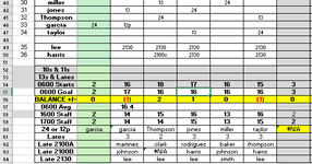
Everyone signs up in column B for Mondays shift and I want to search that column for either 2100B or 2100C and it populate the name that matches that specification in a single cell.
I've attached an example of the spreadsheet I'm working on. Any and all guidance is appreciated.
I'm working on a self-scheduling sheet for a group of 30 employees and I'm trying to figure out how to match two criteria and it populate a single name (index:match type of function except you're matching for possibility of two). Example:
Everyone signs up in column B for Mondays shift and I want to search that column for either 2100B or 2100C and it populate the name that matches that specification in a single cell.
I've attached an example of the spreadsheet I'm working on. Any and all guidance is appreciated.
")


