Matching based on rows

[dhegs]

Hi everyone,

I am looking to create a formula (I am assuming using Index & Match & IF??) that will provide me with a text output (for later use in Pivot Tables) to indicate this data should be removed.

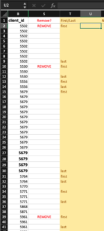
As you can see in the picture, I've already got a column (column S) that refers to many different criteria (in hidden columns) to indicate this data should not be included. As you can see in column B, I have multiple data for each client and column T indicates the "first" and "last" row of this data.

What I am wanting, is to have a formula in column U that will indicate next to "first" and "last" for that client if it should be removed. For example for client 5502 the "first" data indicates it should be removed - I then want it to indicate in column U next to both "first" AND "last" that it should be removed. This will allow me to remove first and last data for this client in the Pivot Table as I can filter for the remove text in column U.

I am hoping someone might be able to help?!

 

[dhegs]

Oh, actually it changed everything , but this should do:

Book1
	B																	S	T	U
2	5502																	REMOVE	first	REMOVE
3	5502
4	5502
5	5502
6	5502																		last	REMOVE
7	5530																		first	REMOVE
8	5530
9	5530																	REMOVE	last	REMOVE
10	1000																		first
11	1000																		last
12	2000																	REMOVE	first	REMOVE
13	2000
14	2000
15	2000
16	2000																		last	REMOVE
17	3000																		first
18	3000
19	3000
20	3000
21	3000																		last
Sheet1

Cell Formulas
Range	Formula
U2:U21	U2	=IF(AND(LEN(T2)>1,ISNUMBER(AGGREGATE(14,6,ROW($B$2:$B$21)/($B$2:$B$21=B2)/NOT(ISBLANK($S$2:$S$21)),1))),"REMOVE","")

[/RANGE

Cell Formulas
Range	Formula

Thank you so much again - your help is so appreciated. Okay so this works... IF column C is just written text, but this is a formula! So I am getting it responding to remove when there is no "REMOVE" because the formula is returning "". I have tried but am unsure how to fix that part of your formula: NOT(ISBLANK($C$2:$C$2325) ?!

 

[Habtest]

Please see the revision:

Book1
	B																	S	T	U
2	5502																	REMOVE	first	REMOVE
3	5502
4	5502
5	5502
6	5502																		last	REMOVE
7	5530																		first	REMOVE
8	5530
9	5530																	REMOVE	last	REMOVE
10	1000																		first
11	1000																		last
12	2000																	REMOVE	first	REMOVE
13	2000
14	2000
15	2000
16	2000																		last	REMOVE
17	3000																		first
18	3000
19	3000
20	3000
21	3000																		last
Sheet1

Cell Formulas
Range	Formula
U2:U21	U2	=IF(AND(LEN(T2)>1,ISNUMBER(AGGREGATE(14,6,ROW($B$2:$B$21)/($B$2:$B$21=B2)/($S$2:$S$21="REMOVE"),1))),"REMOVE","")

I'm still using the table above, including reference to column S instead of C, for consistency purpose. You may of course tweak where needs be.

 

[dhegs]

Please see the revision:

Book1
	B																	S	T	U
2	5502																	REMOVE	first	REMOVE
3	5502
4	5502
5	5502
6	5502																		last	REMOVE
7	5530																		first	REMOVE
8	5530
9	5530																	REMOVE	last	REMOVE
10	1000																		first
11	1000																		last
12	2000																	REMOVE	first	REMOVE
13	2000
14	2000
15	2000
16	2000																		last	REMOVE
17	3000																		first
18	3000
19	3000
20	3000
21	3000																		last
Sheet1

Cell Formulas
Range	Formula
U2:U21	U2	=IF(AND(LEN(T2)>1,ISNUMBER(AGGREGATE(14,6,ROW($B$2:$B$21)/($B$2:$B$21=B2)/($S$2:$S$21="REMOVE"),1))),"REMOVE","")

I'm still using the table above, including reference to column S instead of C, for consistency purpose. You may of course tweak where needs be.

You are a genius! That is great - all tested and all working. Thanks so much again! Apologies for any confusion with using different column letters!

 

[Habtest]

Glad to help, thanks for the feedback