Matching data to bring back a specific rule

PurpleSnow

New Member
Joined
Apr 1, 2022
Messages
3
Office Version
  1. 365
Platform
  1. Windows
Hi All. I'm hoping someone can help me. I need to match data from two separate sources to bring back a specific rule to calculate the carry forward of length of leave.

I have split the calculation into two as its easier to explain it:

Part 1
Source 1
1648803908296.png


Source 2
1648804245255.png

The first part is finding a formula to work out which category the "length of leave" from the green cell in source 1 falls into from source 2.

Part 2
Looking at the example - the category of Length of leave in Source 2 is 3 months +1 day to 6 months.

Now I need a rule that states if the length of leave is 3 months +1 day to 6 months then the number of days/hours carry forward is "14 days/105 hours"

I hope this makes sense?
Thanks
 

Attachments

  • 1648803948341.png
    1648803948341.png
    3.1 KB · Views: 5

Excel Facts

Can you sort left to right?
To sort left-to-right, use the Sort dialog box. Click Options. Choose "Sort left to right"
Welcome to the Board! One idea is shown below. You didn't say if you have the Source 2 table available in an Excel worksheet. Assuming you do, a helper column could be added that describes the lower threshold of each time range in what I'll call the 99ymmdd format. In other words, 99 followed by the number of years of leave, the number of months of leave, and the number of days of leave. Because the number of months and days may have one or two digits, we require that two characters be used for each (e.g., 2 months would be 02). I'm assuming the number of years of leave will rarely exceed 1 (if any?)...and certainly not more than 9, so only one character is needed for years. And in most cases, the number of years will be 0. To avoid an issue where Excel will want to drop this leading 0, I've prepended "99" to the string of numbers (text). So 0 years, 6 months, 18 days of leave would be 9900618. This gives us a number that is readily compared with the lookup Source 2 table, assuming we establish the helper column mentioned above. Then a straightforward XLOOKUP will return the desired result. The primary challenge is creating the number describing the length of leave in 99ymmdd format.

If you are being given the length of leave, then the precise format needs to be known (and preferably consistent). If you are calculating the length of leave in the worksheet, then it would be advantageous to construct the 99ymmdd format directly as each component (years, months, and days) is determined. In this example, I'm assuming you are given (or can be given) the format as "a Y b M c D" and we need to extract a, b, and c from the text string, determine how many characters they are, pad the front of them with a 0 where necessary and finally form the 99ymmdd format. This is the messiest part.

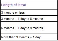
Incidentally, I worked up some formulas for constructing the "a Y b M c D" expression and did not get the same result for the dates in your example (different by two days), but I don't know the details of your calculations (e.g., are holidays, weekends, and perhaps other types of days to be counted). So the primary focus in the following example should begin at cell B7 and then jump to B10 to see how the relevant parts are extracted to create the lookup value. The Source 2 table here includes the lookup column, which is the lower threshold for each bracket expressed in 99ymmdd format. Finally, C10 is the XLOOKUP function that determines which time bracket the lookup value falls within...and the corresponding text from the "Carry forward" column is returned.

If you are not familiar with the XL2BB add-in used to post this working example, you can install it by following the link (see my signature block for a link). You should be able to click on the clipboard copy icon in the upper left of this example (intersection of row/column headings) and paste it into your worksheet (suggested paste into cell A1 to match the same upper left cell as the example)...and then give it a try to see if it returns the expected results.
MrExcel_20220401.xlsx
ABC
1Source 1
2Leave start27/09/2021
3Leave end02/04/2022
4Length of leave:0Y
56M
61D
7Length of leave (one line)0 Y 6 M 1 D
8
9ResultsLength of Leave 99ymmdd formatCarry forward
10990060121 days/157.5 hours
11
12Source 2
13Length of Leave99ymmdd formatMax number of days/hours carry forward
143 months or less99000005 days/37.5 hours
153 months + 1day to 6 months990030114 days/105 hours
166 months + 1 day to 9 months990060121 days/157.5 hours
17more than 9 months + 1 day990090128 days/210 hours
Sheet3
Cell Formulas
RangeFormula
B4B4=DATEDIF($B$2,$B$3,"y")
B5B5=DATEDIF($B$2,$B$3,"ym")
B6B6=$B$3-DATE(YEAR($B$3),MONTH($B$3),1)
B7B7=TEXTJOIN(" ",,B4,C4,B5,C5,B6,C6)
B10B10=LET(y,SEARCH("Y",B7),m,SEARCH("M",B7),d,SEARCH("D",B7),tm,TRIM(MID(B7,y+1,m-y-1 )),td,TRIM(MID(B7,m+1,d-m-1)),VALUE(TEXTJOIN("",,"99",TRIM( LEFT(B7,y-1)),IF(LEN(tm)<2,"0"&tm,tm),IF(LEN(td)<2,"0"&td,td))))
C10C10=XLOOKUP(B10,B14:B17,C14:C17,"not found",-1,1)
 
Upvote 0
Solution
That's good to hear. I'm happy to help. By the way, I just had a look at my Length of Leave calculation and see that there is a problem with it in some cases (for the number of days), plus I neglected to account for the end of the time period (that probably accounts for one of the days of the 2-day discrepancy I mentioned). Assuming your approach for obtaining an expression similar to that shown in B7 (the a Y b M c D text string), the approach I described should work or should be adaptable.
 
Upvote 0
I think the error I mentioned previously is resolved by changing the calculation for days in B6....and a single line version of the Length of Leave formula is shown in C7 (this combines the other Y, M, and D formulas into one formula making the others unnecessary).
MrExcel_20220401.xlsx
ABCD
1Source 1
2Leave start27/09/2021
3Leave end17/03/2022
4Length of leave:0Y
55M
618D
7Length of leave (one line)0 Y 5 M 18 D0 Y 5 M 18 D<-- single line formula
8
9ResultsLength of Leave 99ymmdd formatCarry forward
10990051814 days/105 hours
Sheet3
Cell Formulas
RangeFormula
B4B4=DATEDIF($B$2,$B$3,"y")
B5B5=DATEDIF($B$2,$B$3,"ym")
B6B6=$B$3-EDATE($B$2,12*B4+B5)
B7B7=TEXTJOIN(" ",,B4,C4,B5,C5,B6,C6)
C7C7=LET(y,DATEDIF($B$2,$B$3,"y"),m,DATEDIF($B$2,$B$3,"ym"),d,$B$3-EDATE($B$2,12*y+m),TEXTJOIN(" ",,y,"Y",m,"M",d,"D"))
B10B10=LET(y,SEARCH("Y",B7),m,SEARCH("M",B7),d,SEARCH("D",B7),tm,TRIM(MID(B7,y+1,m-y-1 )),td,TRIM(MID(B7,m+1,d-m-1)),VALUE(TEXTJOIN("",,"99",TRIM( LEFT(B7,y-1)),IF(LEN(tm)<2,"0"&tm,tm),IF(LEN(td)<2,"0"&td,td))))
C10C10=XLOOKUP(B10,B14:B17,C14:C17,"not found",-1,1)
 
Upvote 0

Forum statistics

Threads
1,214,924
Messages
6,122,293
Members
449,077
Latest member
Rkmenon

We've detected that you are using an adblocker.

We have a great community of people providing Excel help here, but the hosting costs are enormous. You can help keep this site running by allowing ads on MrExcel.com.
Allow Ads at MrExcel

Which adblocker are you using?

Disable AdBlock

Follow these easy steps to disable AdBlock

1)Click on the icon in the browser’s toolbar.
2)Click on the icon in the browser’s toolbar.
2)Click on the "Pause on this site" option.
Go back

Disable AdBlock Plus

Follow these easy steps to disable AdBlock Plus

1)Click on the icon in the browser’s toolbar.
2)Click on the toggle to disable it for "mrexcel.com".
Go back

Disable uBlock Origin

Follow these easy steps to disable uBlock Origin

1)Click on the icon in the browser’s toolbar.
2)Click on the "Power" button.
3)Click on the "Refresh" button.
Go back

Disable uBlock

Follow these easy steps to disable uBlock

1)Click on the icon in the browser’s toolbar.
2)Click on the "Power" button.
3)Click on the "Refresh" button.
Go back
Back
Top