merge columns with sorting

[leecavturbo]

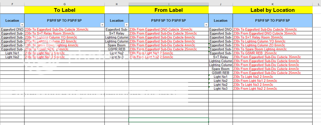
i have 2 columns of data ( label text ) the labels are location specific , the 1st & 3rd column details the location for each. how can my spreadsheet merge the 2 label columns so that the locations are in progressive rows?
so my data is F,G,H,I and i need J,K to auto sort
F is location, G is label, H is location, I is label. J should be location and K label sorted in order of location
TIA

 

[Panda514]

Hello,

Can you give an example of what the first few rows of your data looks like and how you want it to be sorted? You said there are 2 columns of data, but then talked about the 1st and 3rd column. I am having trouble following your description.

 

[leecavturbo]

 

[leecavturbo]

ive manually filled J,K above but need auto fill if poss

 

[leecavturbo]

I can't run Macro's too due to admin rights

 

[Rick Rothstein]

ive manually filled J,K above but need auto fill if poss

Your thread title says "with sorting"... your output column appears to be sorted within each location individually but what determines the order of the locations as they are not sorted alphabetically?

 

[leecavturbo]

Hi Rick, i have manually populated the output column just to show what i should get. no order is required for location if that makes sense

 

[Rick Rothstein]

Hi Rick, i have manually populated the output column just to show what i should get. no order is required for location if that makes sense

I was going to give you a macro solution but I see you posted while I was writing my question to you that you cannot use a macro. I am afraid I do not know how to do what you want with formulas alone. Hopefully one of our formula experts will have a solution for you.

 

[Panda514]

ive manually filled J,K above but need auto fill if poss

I'm not sure if F and H have duplicates, but I would suggest copying all of column F and all of column H into 1 column on another sheet and then using the Remove Duplicates feature on the Data tab to get you a list of each Location. Then you can sort that A to Z if you want and past it into Column J.

For Column K, I have wrote a formula that will lookup the information in G and the lookup the information in I if nothing was found. So basically, for each location it checks in column G then in Column I and returns a blank if nothing is found.

=IFNA(IF(ISNA(VLOOKUP(J3,$F$3:$G$10,2,FALSE)),VLOOKUP(J3,$H$3:$I$10,2,FALSE),1),"")