Merge Multiple Lines into One Cell Reference Noncontiguous Range

[Luke7731]

I have two columns, one with the case number, and the other with varying amount of rows of related case notes (so varying amount of blank rows under each case number). Hundreds of cases, thousands of rows of case notes.
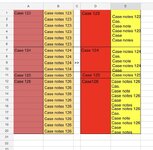
I’ve attached an image of what I have vs what I need. I need the case notes to remain one line on top of the next but I need all of the case notes associated with a case number to be in a single cell next to that case number cell.
So an automated way to merge multiple individual lines of text of various size into a single cell, grouped based on the case numbers to the side.

Thanks!

 

[ACommandLineKindaGuy]

Try this. It assumes your data is in columns A and B on Sheet1 and that you're compiling them onto columns A and B on Sheet2
I also assumed you wanted a line break between each note. I didn't mess with the column width of the compiled notes. You'll probably want it pretty wide

Sub Compile()

Dim i, n As Integer
Dim c As Range

i = 0
n = 0
For Each c In Worksheets(1).Range("A1:A20")    'Modify this to include all the rows with data
If Not IsEmpty(c) Then
        i = i + 1
        n = n + 1
        Worksheets(2).Cells(i, 1) = c.Value
        Worksheets(2).Cells(i, 2) = c.Offset(0, 1).Value
    Else
        n = n + 1
'One of the next 2 lines has to be commented out
        Worksheets(2).Cells(i, 2) = Worksheets(2).Cells(i, 2).Value & vbCrLf & c.Offset(0, 1).Value   'This provides a line break between individual notes.
'        Worksheets(2).Cells(i, 2) = Worksheets(2).Cells(i, 2).Value & " " & c.Offset(0, 1).Value   'This provides a space between individual notes.
    End If
Next c

With Worksheets(2).UsedRange
    .VerticalAlignment = xlTop
    .HorizontalAlignment = xlLeft
End With

End Sub

 

[Peter_SSs]

Hundreds of cases, thousands of rows of case notes.

Given the size of your data, I think this should be much faster.

Sub CaseNotes()
  Dim a As Variant, b As Variant
  Dim i As Long, k As Long
  
  a = Range("A1", Range("B" & Rows.Count).End(xlUp)).Value
  ReDim b(1 To UBound(a), 1 To 2)
  For i = 1 To UBound(a)
    If Len(a(i, 1)) > 0 Then
      k = k + 1
      b(k, 1) = a(i, 1)
      b(k, 2) = a(i, 2)
    Else
      b(k, 2) = b(k, 2) & vbLf & a(i, 2)
    End If
  Next i
  With Range("D1:E1").Resize(k)
    .Columns(2).ColumnWidth = 255
    .Value = b
    .Columns(2).WrapText = True
    .Columns.AutoFit
    .VerticalAlignment = xlTop
  End With
End Sub

Before:

Luke7731.xlsm
	A	B	C	D	E
1	Case 123	Case notes 123
2		Case notes 123
3		Case notes 123
4		Case notes 123
5		Case notes 123
6		Case notes 123
7	Case 124	Case notes 124
8		Case notes 124
9		Case notes 124
10		Case notes 124
11	Case 125	Case notes 125
12	Case 126	Case notes 126
13		Case notes 126
14		Case notes 126
15		Case notes 126
16		Case notes 126
17		Case notes 126
18		Case notes 126
19		Case notes 126
20		Case notes 126
Sheet1

After: (Cols D:E only shown)

Luke7731.xlsm
	D	E
1	Case 123	Case notes 123 Case notes 123 Case notes 123 Case notes 123 Case notes 123 Case notes 123
2	Case 124	Case notes 124 Case notes 124 Case notes 124 Case notes 124
3	Case 125	Case notes 125
4	Case 126	Case notes 126 Case notes 126 Case notes 126 Case notes 126 Case notes 126 Case notes 126 Case notes 126 Case notes 126 Case notes 126
Sheet1

 

[Luke7731]

Given the size of your data, I think this should be much faster.

Sub CaseNotes()
  Dim a As Variant, b As Variant
  Dim i As Long, k As Long
 
  a = Range("A1", Range("B" & Rows.Count).End(xlUp)).Value
  ReDim b(1 To UBound(a), 1 To 2)
  For i = 1 To UBound(a)
    If Len(a(i, 1)) > 0 Then
      k = k + 1
      b(k, 1) = a(i, 1)
      b(k, 2) = a(i, 2)
    Else
      b(k, 2) = b(k, 2) & vbLf & a(i, 2)
    End If
  Next i
  With Range("D1:E1").Resize(k)
    .Columns(2).ColumnWidth = 255
    .Value = b
    .Columns(2).WrapText = True
    .Columns.AutoFit
    .VerticalAlignment = xlTop
  End With
End Sub

Before:

Luke7731.xlsm
	A	B	C	D	E
1	Case 123	Case notes 123
2		Case notes 123
3		Case notes 123
4		Case notes 123
5		Case notes 123
6		Case notes 123
7	Case 124	Case notes 124
8		Case notes 124
9		Case notes 124
10		Case notes 124
11	Case 125	Case notes 125
12	Case 126	Case notes 126
13		Case notes 126
14		Case notes 126
15		Case notes 126
16		Case notes 126
17		Case notes 126
18		Case notes 126
19		Case notes 126
20		Case notes 126
Sheet1

After: (Cols D:E only shown)

Luke7731.xlsm
	D	E
1	Case 123	Case notes 123 Case notes 123 Case notes 123 Case notes 123 Case notes 123 Case notes 123
2	Case 124	Case notes 124 Case notes 124 Case notes 124 Case notes 124
3	Case 125	Case notes 125
4	Case 126	Case notes 126 Case notes 126 Case notes 126 Case notes 126 Case notes 126 Case notes 126 Case notes 126 Case notes 126 Case notes 126
Sheet1

This worked wonderfully, thank you

 

[Luke7731]

Try this. It assumes your data is in columns A and B on Sheet1 and that you're compiling them onto columns A and B on Sheet2
I also assumed you wanted a line break between each note. I didn't mess with the column width of the compiled notes. You'll probably want it pretty wide

Sub Compile()

Dim i, n As Integer
Dim c As Range

i = 0
n = 0
For Each c In Worksheets(1).Range("A1:A20")    'Modify this to include all the rows with data
If Not IsEmpty(c) Then
        i = i + 1
        n = n + 1
        Worksheets(2).Cells(i, 1) = c.Value
        Worksheets(2).Cells(i, 2) = c.Offset(0, 1).Value
    Else
        n = n + 1
'One of the next 2 lines has to be commented out
        Worksheets(2).Cells(i, 2) = Worksheets(2).Cells(i, 2).Value & vbCrLf & c.Offset(0, 1).Value   'This provides a line break between individual notes.
'        Worksheets(2).Cells(i, 2) = Worksheets(2).Cells(i, 2).Value & " " & c.Offset(0, 1).Value   'This provides a space between individual notes.
    End If
Next c

With Worksheets(2).UsedRange
    .VerticalAlignment = xlTop
    .HorizontalAlignment = xlLeft
End With

End Sub

Thank you!

 

[ACommandLineKindaGuy]

Sorry--I misread your initial post. Here's a mini-sheet that explains the process. You can hide the substatus list column if you like, but you must keep it populated alongside your main tabulation data validation rows.

Cascading Dropdowns.xlsx
	A	B	C	D	E	F
1	Lead	Status	SubStatus	Substatus List		Won
2	B	Lost		LostB		Won
3	A	Won		Won
4				NA		LostA
5				NA		The client has already signed the offer (I arrived too late)
6				NA		Unsigned agreement
7				NA		The client did not send any information
8				NA		Choose another offer
9				NA		There is no solution for the client's request
10				NA
11				NA		LostB
12				NA		Unsigned agreement
13				NA		The client did not send any information
14				NA		Choose another offer
15				NA		There is no solution for the client's request
16				NA		The client does not have a specific request for GrECo
17				NA
18				NA		Pending
19				NA		Insufficient contact details
20				NA		The signed brokerage contract was awaited
21	END OF TABLE					We are waiting for information from the client for the offer
22						Offer sent
23						We are waiting for a response to the offer
24						A meeting with the client was requested
Sheet1

Cell Formulas
Range	Formula
D2:D20	D2	=IF(B2="Lost","Lost"&A2,IF(B2="Won","Won",IF(B2="Pending","Pending","NA")))

Cells with Data Validation
Cell	Allow	Criteria
A2:A20	List	A,B
B2:B20	List	Won,Lost,Pending
C2:C20	List	=INDIRECT(D2)

 

[Luke7731]

This worked wonderfully, thank you

So when I use it on a shorter sampe of my data it works great, but when I apply it to the whole dataset I get this error. Im not exactly sure what my problem is or how to go about fixing it. Lots of data accumulated by various secretaries over the years.
Thanks

 

[Luke7731]

Given the size of your data, I think this should be much faster.

Sub CaseNotes()
  Dim a As Variant, b As Variant
  Dim i As Long, k As Long
 
  a = Range("A1", Range("B" & Rows.Count).End(xlUp)).Value
  ReDim b(1 To UBound(a), 1 To 2)
  For i = 1 To UBound(a)
    If Len(a(i, 1)) > 0 Then
      k = k + 1
      b(k, 1) = a(i, 1)
      b(k, 2) = a(i, 2)
    Else
      b(k, 2) = b(k, 2) & vbLf & a(i, 2)
    End If
  Next i
  With Range("D1:E1").Resize(k)
    .Columns(2).ColumnWidth = 255
    .Value = b
    .Columns(2).WrapText = True
    .Columns.AutoFit
    .VerticalAlignment = xlTop
  End With
End Sub

Before:

Luke7731.xlsm
	A	B	C	D	E
1	Case 123	Case notes 123
2		Case notes 123
3		Case notes 123
4		Case notes 123
5		Case notes 123
6		Case notes 123
7	Case 124	Case notes 124
8		Case notes 124
9		Case notes 124
10		Case notes 124
11	Case 125	Case notes 125
12	Case 126	Case notes 126
13		Case notes 126
14		Case notes 126
15		Case notes 126
16		Case notes 126
17		Case notes 126
18		Case notes 126
19		Case notes 126
20		Case notes 126
Sheet1

After: (Cols D:E only shown)

Luke7731.xlsm
	D	E
1	Case 123	Case notes 123 Case notes 123 Case notes 123 Case notes 123 Case notes 123 Case notes 123
2	Case 124	Case notes 124 Case notes 124 Case notes 124 Case notes 124
3	Case 125	Case notes 125
4	Case 126	Case notes 126 Case notes 126 Case notes 126 Case notes 126 Case notes 126 Case notes 126 Case notes 126 Case notes 126 Case notes 126
Sheet1

So when I use it on a shorter sampe of my data it works great, but when I apply it to the whole dataset I get this error. Im not exactly sure what my problem is or how to go about fixing it. Lots of data accumulated by various secretaries over the years.
Thanks

 

[Peter_SSs]

Could you have error values in your data?

When you get the error, click Debug and then hover over the variable i:

Whatever number shows in the pop-up, go to that row in your data and look at the value in column B of that row.

 

[Georgiboy]

I was playing with a formula:

Book1
	A	B	C	D	E
1				123	Case notes 123 Case notes 123 Case notes 123 Case notes 123 Case notes 123 Case notes 123
2				124	Case notes 124 Case notes 124 Case notes 124 Case notes 124
3				125	Case notes 125
4				126	Case notes 126 Case notes 126 Case notes 126 Case notes 126 Case notes 126 Case notes 126 Case notes 126 Case notes 126 Case notes 126
5	123	Case notes 123
6		Case notes 123
7		Case notes 123
8		Case notes 123
9		Case notes 123
10		Case notes 123
11	124	Case notes 124
12		Case notes 124
13		Case notes 124
14		Case notes 124
15	125	Case notes 125
16	126	Case notes 126
17		Case notes 126
18		Case notes 126
19		Case notes 126
20		Case notes 126
21		Case notes 126
22		Case notes 126
23		Case notes 126
24		Case notes 126
Sheet1

Cell Formulas
Range	Formula
D1:E4	D1	=LET(a,$A$5:$A$24,b,$B$5:$B$24,c,ROW(a),u,UNIQUE(LOOKUP(ROW(a),IF(LEN(a),ROW(a)), a)),HSTACK(u,BYROW(u,LAMBDA(br,TEXTJOIN(CHAR(10),,FILTER(b,LOOKUP(c,IF(LEN(a),c), a)=br))))))
Dynamic array formulas.