MIN/MAXIFS function with a criteria that returns multiple correct answers

[Mikek1988]

Hi everyone,

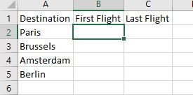
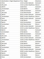
I am trying to use some data to find the minimum and maximum values using the MINIFS and MAXIFS function.
However one of my criteria needs to have multiple answers, so the answer of a range could be 'A' or 'B' etc

So far I have got it to return an result for one answer but I also need it to look up other values too as they could be the correct answer instead.

I cannot upload the sheet because it is confidential, any ideas would be greatly appreciated

 

[Eric W]

When the result of a formula in Excel 365 is an array, it will SPILL all the individual answers in multiple cells, which is what you're seeing in the H2 formula. If you get a 0 when you use MIN on that, it must mean that one of the individual results is 0.

It sounds like you want multiple answers on multiple rows, using some other criteria. Can you show what you're seeing with a screen print? What you have and the desired results? The XL2BB tool which I used in posts 3 and 5 is easy to download, install and use. See the link in my signature or the reply box. Dummy up some fake data if there's anything sensitive.

Or you can just copy and paste a section of your sheet into the reply box, but you'll also need to show me the formula you're using.

 

[Mikek1988]

Attached are some pictures of a basic version of a spreadsheet similar to mine,
Example 1 shows the raw data which contains flights to and from locations with their departure times and their direction, from this the earliest flight and the latest flight to each destination needs to be shown but it has to look at the origin airports (in my version this is essential) and it also has to look up the direction,

So the equation i have been trying to use is for the earliest flight:
= MINIFS (
the possible times is the next part, Example1!B2:B30,
the next part is the first criteria which is to look up certain airports so now i tried, Example1!C2:C30,{"London Gatwick","Paris","Berlin"}
the next part is the possible destination airports, Example1!A2:A30,Example2!A2:A5
the last part is the direction, Example1!D2:D30, "Outward"

so when i have it constructed it looks like this

=MINIFS(Example1!B2:B30,Example1!C2:C30,{"London Gatwick","Paris","Berlin"},Example1!A2:A30,Example2!A2:A5,Example1!D2:D30,"Outward")

but for some reason it doesnt work or doesnt come up with any results, is there a way i can achieve what i need?

 

[Mikek1988]

When the result of a formula in Excel 365 is an array, it will SPILL all the individual answers in multiple cells, which is what you're seeing in the H2 formula. If you get a 0 when you use MIN on that, it must mean that one of the individual results is 0.

It sounds like you want multiple answers on multiple rows, using some other criteria. Can you show what you're seeing with a screen print? What you have and the desired results? The XL2BB tool which I used in posts 3 and 5 is easy to download, install and use. See the link in my signature or the reply box. Dummy up some fake data if there's anything sensitive.

Or you can just copy and paste a section of your sheet into the reply box, but you'll also need to show me the formula you're using.

Hi,

Sorry i dont think my work laptop is allowing me to install XL2BB so ive had to post the pics above

 

[Eric W]

The reason you're getting 0 is because you're giving the formula a list of origins for column C, and giving it a list of destinations for column A. Some of those airports are the same. The MAXIFS is looking at every combination of those 2 lists, including combinations like Paris -> Paris and Berlin -> Berlin. For those combinations, it won't find any flights, so the MIN for those combinations is 0, making the overall MIN also 0.

If the destination is Paris, do you care what the origin is? If not, the basic B2 formula below should work. Put it in B2 and drag down. If you do have a list of acceptable origins that is the same for your entire list, you'd have to ratchet up the difficulty level a bit to the C2 formula.

Book2
	A	B	C
1	Destination	First Flight	First Flight
2	Paris	9:00	9:00
3	Brussels	No flight	No flight
4	Amsterdam	No flight	No flight
5	Berlin	9:15	9:15
6
Example2

Cell Formulas
Range	Formula
B2:B5	B2	=IFERROR(1/(1/MINIFS(Example1!$B$2:$B$10,Example1!$A$2:$A$10,A2,Example1!$D$2:$D$10,"Outward")),"No flight")
C2:C5	C2	=IFERROR(SMALL(IFERROR(1/(1/MINIFS(Example1!$B$2:$B$10,Example1!$A$2:$A$10,A2,Example1!$D$2:$D$10,"Outward",Example1!$C$2:$C$10,{"London Gatwick","Paris","Berlin"})),""),1),"No flight")

 

[Mikek1988]

The reason you're getting 0 is because you're giving the formula a list of origins for column C, and giving it a list of destinations for column A. Some of those airports are the same. The MAXIFS is looking at every combination of those 2 lists, including combinations like Paris -> Paris and Berlin -> Berlin. For those combinations, it won't find any flights, so the MIN for those combinations is 0, making the overall MIN also 0.

If the destination is Paris, do you care what the origin is? If not, the basic B2 formula below should work. Put it in B2 and drag down. If you do have a list of acceptable origins that is the same for your entire list, you'd have to ratchet up the difficulty level a bit to the C2 formula.

Book2
	A	B	C
1	Destination	First Flight	First Flight
2	Paris	9:00	9:00
3	Brussels	No flight	No flight
4	Amsterdam	No flight	No flight
5	Berlin	9:15	9:15
6
Example2

Cell Formulas
Range	Formula
B2:B5	B2	=IFERROR(1/(1/MINIFS(Example1!$B$2:$B$10,Example1!$A$2:$A$10,A2,Example1!$D$2:$D$10,"Outward")),"No flight")
C2:C5	C2	=IFERROR(SMALL(IFERROR(1/(1/MINIFS(Example1!$B$2:$B$10,Example1!$A$2:$A$10,A2,Example1!$D$2:$D$10,"Outward",Example1!$C$2:$C$10,{"London Gatwick","Paris","Berlin"})),""),1),"No flight")

Hi,

Sorry my example was a quick and dirty and should have checked for same origin and destination, in mine they won't be the same and very rarely there will be a zero answer.

In the Paris example not every origin will go there but I need to search only for specific origins to check if there is a flight in case there is an earlier one that would count.

I will try your equations in the morning and see how it goes, thanks for your ongoing help

 

[Mikek1988]

The reason you're getting 0 is because you're giving the formula a list of origins for column C, and giving it a list of destinations for column A. Some of those airports are the same. The MAXIFS is looking at every combination of those 2 lists, including combinations like Paris -> Paris and Berlin -> Berlin. For those combinations, it won't find any flights, so the MIN for those combinations is 0, making the overall MIN also 0.

If the destination is Paris, do you care what the origin is? If not, the basic B2 formula below should work. Put it in B2 and drag down. If you do have a list of acceptable origins that is the same for your entire list, you'd have to ratchet up the difficulty level a bit to the C2 formula.

Book2
	A	B	C
1	Destination	First Flight	First Flight
2	Paris	9:00	9:00
3	Brussels	No flight	No flight
4	Amsterdam	No flight	No flight
5	Berlin	9:15	9:15
6
Example2

Cell Formulas
Range	Formula
B2:B5	B2	=IFERROR(1/(1/MINIFS(Example1!$B$2:$B$10,Example1!$A$2:$A$10,A2,Example1!$D$2:$D$10,"Outward")),"No flight")
C2:C5	C2	=IFERROR(SMALL(IFERROR(1/(1/MINIFS(Example1!$B$2:$B$10,Example1!$A$2:$A$10,A2,Example1!$D$2:$D$10,"Outward",Example1!$C$2:$C$10,{"London Gatwick","Paris","Berlin"})),""),1),"No flight")

Hi,

Thanks for your help C2 worked great

Is there a way to apply a countif instead of min and maxifs as well?

 

[Eric W]

Yes, the basic idea is to use SUM(COUNTIFS(... and set up the COUNTIFS like the MINIFS. Let me know if you have questions.