MINIFS Conditional formatting

JARichard74

Board Regular
Joined
Dec 16, 2019
Messages
114
Office Version
  1. 365
Platform
  1. Windows
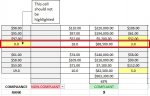
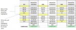
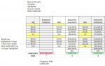
In conditional formatting, this formula =AND(G4=MINIFS($G4:$Y4,$H$16:$Z$16,"COMPLIANT"),G4<>"") is applied to =$G$4:$G$13,$I$4:$I$13,$K$4:$K$13,$Y$4:$Y$13,$W$4:$W$13,$U$4:$U$13,$S$4:$S$13,$Q$4:$Q$13,$O$4:$O$13,$M$4:$M$13. It highlights the minimum value if the cell is not blank and H:Z is COMPLIANT. It works perfectly except for when a value in the G:Y range = 0. If I change H:Z value then the next lowest values gets highlighted as I want however, the 0 also stays highlighted. Any assistance would be appreciated.
 

Attachments

  • Clipboard01.jpg
    Clipboard01.jpg
    40.3 KB · Views: 42

Excel Facts

Workdays for a market open Mon, Wed, Friday?
Yes! Use "0101011" for the weekend argument in NETWORKDAYS.INTL or WORKDAY.INTL. The 7 digits start on Monday. 1 means it is a weekend.
=AND(G4=MINIFS($G4:$Y4,$H$16:$Z$16,"COMPLIANT"),G4<>"",G4<>0)
 
Upvote 0
From what I can see the the 2 parts of the formula will be conflicting each other, try doing it without AND

=G4=MINIFS($G4:$Y4,$G4:$Y4,"<>0",$H$16:$Z$16,"COMPLIANT")
 
Upvote 0
Wayne(etaf), your suggestion produces the same result. Jason, yours does not ignore blank cells. I also have to be careful about ignoring 0 as it is a valid response in my current context
 
Upvote 0
Your post implied that 0 should not be highlighted, if you only want to ignore blanks then try.

=G4=MINIFS($G4:$Y4,$G4:$Y4,"<>",$H$16:$Z$16,"COMPLIANT")
 
Upvote 0
Still highlights empty cells (See Image 1). When I move $H$16:$Z$16 to something other than COMPLIANT then none of the cells in G4:G13 should be highlighted as they should be excluded from the MIN (See image 2)
 

Attachments

  • Image 1.jpg
    Image 1.jpg
    64.4 KB · Views: 12
  • Image 2.jpg
    Image 2.jpg
    68.3 KB · Views: 11
Upvote 0
what range have you chosen ?
Book4
GHIJKLM
1FALSEFALSETRUEFALSEFALSE
2
3
41098
5
6
7
8
9
10
11
12
13
14
15
16compliantcompliantcompliant
17
18
Sheet1
Cell Formulas
RangeFormula
G1:K1G1=AND(G4=MINIFS($G4:$Y4,$H$16:$Z$16,"COMPLIANT"),G4<>"",G4<>0)
Cells with Conditional Formatting
CellConditionCell FormatStop If True
G4:M16Expression=AND(G4=MINIFS($G4:$Y4,$H$16:$Z$16,"COMPLIANT"),G4<>"",G4<>0)textNO
 
Upvote 0
I was getting mixed up on the absolute and relative ranges, this should be bulletproof.

=AND(G4<>"",H$16="COMPLIANT",G4=MINIFS($G4:$Y4,$G4:$Y4,"<>",$H$16:$Z$16,"COMPLIANT"))
 
Upvote 0
Solution
Thanks Jason, this seems to have done the trick!
Wayne, in your example I am only evaluating every second column for the MIN i.e. G,I,K,M,O,Q,S,U,W,Y
 
Upvote 0

Forum statistics

Threads
1,214,922
Messages
6,122,281
Members
449,075
Latest member
staticfluids

We've detected that you are using an adblocker.

We have a great community of people providing Excel help here, but the hosting costs are enormous. You can help keep this site running by allowing ads on MrExcel.com.
Allow Ads at MrExcel

Which adblocker are you using?

Disable AdBlock

Follow these easy steps to disable AdBlock

1)Click on the icon in the browser’s toolbar.
2)Click on the icon in the browser’s toolbar.
2)Click on the "Pause on this site" option.
Go back

Disable AdBlock Plus

Follow these easy steps to disable AdBlock Plus

1)Click on the icon in the browser’s toolbar.
2)Click on the toggle to disable it for "mrexcel.com".
Go back

Disable uBlock Origin

Follow these easy steps to disable uBlock Origin

1)Click on the icon in the browser’s toolbar.
2)Click on the "Power" button.
3)Click on the "Refresh" button.
Go back

Disable uBlock

Follow these easy steps to disable uBlock

1)Click on the icon in the browser’s toolbar.
2)Click on the "Power" button.
3)Click on the "Refresh" button.
Go back
Back
Top