Multi Criteria Match Problem ...

[Russ At Index]

Hello , out in the Greater Excel World ,

Once again i find myself reaching out for some kind assistance on a project .

Overview being i want to populate a spreadsheet with a specific number that relates to all the criteria held in both spreadsheets, so here goes with my
explanation .

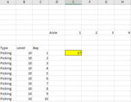
Sheet1 Cells have :
A10 - Type
B10 - Level
C10 - Bay
E6 - Aisle
My answer will sit in cell E10 & be copied to populate the data in sheet 1

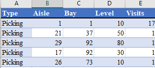
Sheet2 has a table which following data sits :
Column A - Type
Column B - Aisle
Column C - Bay
Column D - Level
Column G - Contains the number which i need to populate E6 with in sheet 1

Any solution would be greatly appreciated ,

Stay safe ,

Russ.

 

[Russ At Index]

Hi ,

Any ideas , would attaching screen shot of my issue help in any way ?.

Thanks ,

Russ.

 

[Peter_SSs]

would attaching screen shot of my issue help in any way ?

Yes, especially if it includes the expected results and is provided with XL2BB so helpers would not have to manually type out the data to test with.

 

[Russ At Index]

Hi Peter ,

Thanks for your reply,
Sheet 1 Sheet 2
.

Result answer =17 is highlighted where i hope the formula will sit !

Stay safe ,

Russ.

 

[Peter_SSs]

Any chance of this?

with XL2BB so helpers would not have to manually type out the data to test with.

What is the name of the table in Sheet2?

Does this have to work in both Excel 365 and 2016 or would 365 only be okay?

 

[stigcorneer]

If you only have uniqe sets of Aisle-Bay-Level combinations in Table on Sheet2you could use a SUMIFS()

E10 =SUMIFS(Table[Visits],Table[Aisle],E$6,Table[Bay],$C10,Table[Level],$B10)

 

[Russ At Index]

Hi Peter ,

365 & TableVisits

 

[Russ At Index]

If you only have uniqe sets of Aisle-Bay-Level combinations in Table on Sheet2you could use a SUMIFS()

E10 =SUMIFS(Table[Visits],Table[Aisle],E$6,Table[Bay],$C10,Table[Level],$B10)

Hi Stig
All information on table is numerical and related to the layout of a warehouse, does that help atall ?.
Tahnks fo ryour time,
Russ

 

[Peter_SSs]

See if this does what you want. Note that I have altered the sample data a little.
I have also assumed unique sets of Type/Aisle/Bay/Level in the Sheet2 table.

Russ At Index.xlsm
	A	B	C	D	E
1	Type	Aisle	Bay	Level	Visits
2	Picking	1	1	10	17
3	Picking	3	5	50	1
4	Picking	5	3	10	122
5	Picking	8	2	10	1
6	Picking	6	73	10	1
Sheet2

Formula in E10 is copied across and down

Russ At Index.xlsm
	A	B	C	D	E	F	G	H	I	J	K	L	M
6				Aisle	1	2	3	4	5	6	7	8	9
7
8
9	Type	Level	Bay
10	Picking	10	1		17
11	Picking	10	2									1
12	Picking	10	3						122
13	Picking	10	4
14	Picking	10	5
15	Picking	10	6
16	Picking	10	7
17	Picking	10	8
Sheet1

Cell Formulas
Range	Formula
E10:M17	E10	=INDEX(FILTER(TableVisits[[Visits]:[Visits]],(TableVisits[[Type]:[Type]]=$A10)*(TableVisits[[Aisle]:[Aisle]]=E$6)*(TableVisits[[Bay]:[Bay]]=$C10)*(TableVisits[[Level]:[Level]]=$B10),""),1)

 

[Russ At Index]

See if this does what you want. Note that I have altered the sample data a little.
I have also assumed unique sets of Type/Aisle/Bay/Level in the Sheet2 table.

Russ At Index.xlsm
	A	B	C	D	E
1	Type	Aisle	Bay	Level	Visits
2	Picking	1	1	10	17
3	Picking	3	5	50	1
4	Picking	5	3	10	122
5	Picking	8	2	10	1
6	Picking	6	73	10	1
Sheet2

Formula in E10 is copied across and down

Russ At Index.xlsm
	A	B	C	D	E	F	G	H	I	J	K	L	M
6				Aisle	1	2	3	4	5	6	7	8	9
7
8
9	Type	Level	Bay
10	Picking	10	1		17
11	Picking	10	2									1
12	Picking	10	3						122
13	Picking	10	4
14	Picking	10	5
15	Picking	10	6
16	Picking	10	7
17	Picking	10	8
Sheet1

Cell Formulas
Range	Formula
E10:M17	E10	=INDEX(FILTER(TableVisits[[Visits]:[Visits]],(TableVisits[[Type]:[Type]]=$A10)*(TableVisits[[Aisle]:[Aisle]]=E$6)*(TableVisits[[Bay]:[Bay]]=$C10)*(TableVisits[[Level]:[Level]]=$B10),""),1)

Hi Peter ,

Thank you for your kind assistance , i will try the formula in due course & let you know the outcome,

Many thanks ,

Russ.