Multi-dimensional INDEX/MATCH using the table ROW and COLUMN headers to search

[logic]

I am using Excel to calculate pricing using 2 tables:

A retail pricing list
A distributor discount list

The distributors discount is variable, and therefore, in a third table, I am trying to calculate the pricing.

I would like to use the table row label and table column label to refer to the retail pricing list.

Currently I am using INDEX/MATCH to do this:

{=INDEX(retail_price_list_price,MATCH(1,(A1=retail_price_list_type)*(B1=retail_price_list_material)*(C1=retail_price_list_color),0)))*(100-distributor_discount_percentage)

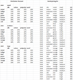
So, as an example, a shirt that is small and violet and polyester should reference to value in the '300' in the 'retail pricing list'

In the third table, I should automatically get the value of 255, the price at which the distributor would buy from us.

Now, the question is: I have 70 tables for the distributor discount. Manually doing the formulas for close to 10000 lines is not a good use of my time.

So, how would I have excel search by finding the discount at the intersection of material (silk/cotton/polyester/wool) and color (violet/indigo/blue/green/yellow/orange/red) without me changing every cell reference when I paste it for the third table? I don't mind pasting it 70 times, but changing the values close to 10000 times is a bit much.

 

[Legacy 143009]

It is very hard to tell me in English I am directly sharing the example. You should write this formula just as the substitute for the underlined statement. The rest will be the same:
{=INDEX(retail_price_list_price,MATCH(1,(A1=retail_price_list_type)*(B1=retail_price_list_material)*(C1=retail_price_list_color),0)))*(100-distributor_discount_percentage)

=INDEX(INDEX(D:D,MATCH(1,(D1:D18="shirt")*(E1:E18="medium"),0)):H18,MATCH("green",INDEX(D:D,MATCH(1,(D1:D18="shirt")*(E1:E18="medium"),0)):D18,0),MATCH("cotton",INDEX(INDEX(D:D,MATCH(1,(D1:D18="shirt")*(E1:E18="medium"),0)+1),INDEX(H:H,MATCH(1,(D1:D18="shirt")*(E1:E18="medium"),0)+1),0)))

I hope you can manage to modify it according to your data.