Multiple Column - Multiple Value Costing

[Jennifer Meyer]

Good morning,
I have a worksheet generated from another program that does not list our opening numbers in a way that I can find total cost for one opening at at time.

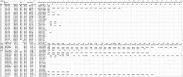
The worksheet has 57 columns of "Openings", inside these columns are 1483 opening #'s and each opening # may be found many times in different rows. The rows for each opening #'s is the cost for that part of the opening. I need to find a total cost for each opening.

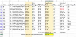
I tried many different formulas and arrangements to be able to enter/find/sort 1 opening # from the worksheet and have it sum all associated (row costs) and could not get anything to work. I have also attached an image (Opening Costs Complete - by Opening) that I made by doing hours of cutting/pasting, and inserting rows to get all 1483 openings (from each of the 57 columns) to Column J. I inserted rows and then copied down the costs. As you can see by Row 1488/Column J, I have a formula that calculates the Net Cost after filtering by Opening #.

I know that excel is very powerful and believe there is a better way. I have to pull this report from our program frequently for different projects so I am looking to find a faster way to convert my file "Cost by Opening numbers" to what I created manually "Openings Costs Complete".

Please help!
Jennifer

 

[StephenCrump]

Perhaps something like this:

	A	B	C	D	E	F	G	H	I	J	K	L
1	Product	Cost	Open 1	Open 2	Open 3	Open 4	Open 5	Open 6	Open 7	Open 8	Open 9	Open 10
2	A	$3.00	999	999	999	111
3	B	$1.00	999
4	C	$1.00	999
5	D	$5.00	999	999	999	999	999	999	999	111
6	E	$1.00	999
7	F	$1.00	999
8	G	$1.00	999	999
9	H	$7.00	999	999	111
10	I	$1.00	999	999
11	J	$1.00	999
12	K	$1.00	999
13
14
15	Total for	111
16		$15.00
Sheet1

Cell Formulas
Range	Formula
B16	B16	=SUM(IF(MMULT(--(C2:L12=B15),TRANSPOSE(COLUMN(C1:L1)^0)),B2:B12))

(You'll need to array enter this formula).

 

[Jennifer Meyer]

Perhaps something like this:

	A	B	C	D	E	F	G	H	I	J	K	L
1	Product	Cost	Open 1	Open 2	Open 3	Open 4	Open 5	Open 6	Open 7	Open 8	Open 9	Open 10
2	A	$3.00	999	999	999	111
3	B	$1.00	999
4	C	$1.00	999
5	D	$5.00	999	999	999	999	999	999	999	111
6	E	$1.00	999
7	F	$1.00	999
8	G	$1.00	999	999
9	H	$7.00	999	999	111
10	I	$1.00	999	999
11	J	$1.00	999
12	K	$1.00	999
13
14
15	Total for	111
16		$15.00
Sheet1

Cell Formulas
Range	Formula
B16	B16	=SUM(IF(MMULT(--(C2:L12=B15),TRANSPOSE(COLUMN(C1:L1)^0)),B2:B12))

(You'll need to array enter this formula).

Perhaps something like this:

	A	B	C	D	E	F	G	H	I	J	K	L
1	Product	Cost	Open 1	Open 2	Open 3	Open 4	Open 5	Open 6	Open 7	Open 8	Open 9	Open 10
2	A	$3.00	999	999	999	111
3	B	$1.00	999
4	C	$1.00	999
5	D	$5.00	999	999	999	999	999	999	999	111
6	E	$1.00	999
7	F	$1.00	999
8	G	$1.00	999	999
9	H	$7.00	999	999	111
10	I	$1.00	999	999
11	J	$1.00	999
12	K	$1.00	999
13
14
15	Total for	111
16		$15.00
Sheet1

Cell Formulas
Range	Formula
B16	B16	=SUM(IF(MMULT(--(C2:L12=B15),TRANSPOSE(COLUMN(C1:L1)^0)),B2:B12))

(You'll need to array enter this formula).

Thank you!

I have found antoher problem and it is not related to your formula. Unfortunately the program groups some of the openings together like G202(2), this means there are two of the G202. I have many instances of these single cell values like this. Is there a formula to get these values into there own separate cells or to account for them for the value in the parenthesis? I have to account for these this value as 2 openings, not just one. Because of these cells my costs per opening is not calculating completely. Values like this G202(2), 111(3), etc are throughout many columns in my worksheet.

Jennifer

 

[StephenCrump]

Perhaps:

	A	B	C	D	E	F	G	H	I	J	K	L
1	Product	Cost	1	2	3	4	5	6	7	8	9	10
2	A	3	999	999	999	111
3	B	1	999
4	C	1	999
5	D	5	999	999	999	999	999	999	999	111(2)
6	E	1	999
7	F	1	999
8	G	1	999	999
9	H	7	999	999	111 (3)
10	I	1	999	999
11	J	1	999
12	K	1	999
13
14
15	Total for	111
16		15
Sheet1

Cell Formulas
Range	Formula
B16	B16	=SUM(IF(MMULT(--(TEXT(IFERROR(TRIM(LEFT(C2:L12,FIND("(",C2:L12)-1)),C2:L12),"0")=TEXT(B15,"0")),TRANSPOSE(COLUMN(C1:L1)^0)),B2:B12))

This assumes that the only "(" character in your code will identify duplicates, and that you want to ignore everything after the "(".

If you codes can include, say 123 (large) and 123 (large)(2) then we'll need to modify the approach.

EDIT: Sorry, I just re-read your question and may be misinterpreting. In the example above, is the answer supposed to be:
3 + (5 x 2) +( 7 x 3) = 34?

 

[StephenCrump]

EDIT: Sorry, I just re-read your question and may be misinterpreting. In the example above, is the answer supposed to be:
3 + (5 x 2) +( 7 x 3) = 34?

In which case ..

	A	B	C	D	E	F	G	H	I	J	K	L
1	Product	Cost	1	2	3	4	5	6	7	8	9	10
2	A	3	999	999	999	111
3	B	1	999
4	C	1	999
5	D	5	999	999	999	999	999	999	999	111(2)
6	E	1	999
7	F	1	999
8	G	1	999	999
9	H	7	999	999	111 (3)	111 (7)
10	I	1	999	999
11	J	1	999
12	K	1	999
13
14
15	Total for	111
16		83
Sheet1

Cell Formulas
Range	Formula
B16	B16	=SUM(MMULT((TEXT(IFERROR(TRIM(LEFT(Openings,FIND("(",Openings)-1)),Openings),"0")=TEXT(B15,"0"))*IFERROR(-RIGHT(C2:L12,LEN(Openings)-FIND("(",Openings)+1),1),TRANSPOSE(COLUMN(C1:L1)^0))*Cost)

Named Ranges
Name	Refers To	Cells
Cost	=Sheet1!$B$2:$B$12	B16
Openings	=Sheet1!$C$2:$L$12	B16

 

[Jennifer Meyer]

Thank you!

Jennifer

 

[Jennifer Meyer]

I have one more request of this formula or for an add to my worksheet. Sometimes the openings are "phased" and we are asked for "phasing" costs, is it possible?

In your example, if values in C2-J12 are each in a different "phase", can I get a cost by phase if I have a list of opening and corresponding phase? Is there a way to look for through all the openings, match those with the a list of total opening to get what phase they are in and get a cost by phase?

 

[StephenCrump]

I haven't provided formulas yet - just checking this is what you mean?

	A	B	C	D	E	F	G	H	I	J	K	L	M
1	Product	Phase	Cost	1	2	3	4	5	6	7	8	9	10
2	A	1	$3	999	999	999	111
3	B	1	$1	999
4	C	1	$1	999
5	D	1	$5	999	999	999	999	999	999	999	111(2)
6	E	1	$1	999
7	F	1	$1	999
8	G	1	$1	999	999
9	H	2	$7	999	999	111 (3)	111 (7)
10	I	1	$1	999	999
11	J	1	$1	999
12	K	1	$1	999
13
14
15	Totals for:		111
16	Phase	1	$13
17		2	$70
Sheet6

 

[Jennifer Meyer]

Sorry for the delay, we got busy and this project got put to the back burner.

Yes, I think so. I want to be able to search all #'s columns D-L for a number, match that to a phase on a different worksheet, then total the costs. My #s in the D-L columns will only be in one Phase, not like you show 111 in Phase 1 and Phase 2. My phases and Items # will be on another work sheet.

Jennifer

 

[Jennifer Meyer]

I haven't provided formulas yet - just checking this is what you mean?

	A	B	C	D	E	F	G	H	I	J	K	L	M
1	Product	Phase	Cost	1	2	3	4	5	6	7	8	9	10
2	A	1	$3	999	999	999	111
3	B	1	$1	999
4	C	1	$1	999
5	D	1	$5	999	999	999	999	999	999	999	111(2)
6	E	1	$1	999
7	F	1	$1	999
8	G	1	$1	999	999
9	H	2	$7	999	999	111 (3)	111 (7)
10	I	1	$1	999	999
11	J	1	$1	999
12	K	1	$1	999
13
14
15	Totals for:		111
16	Phase	1	$13
17		2	$70
Sheet6

Sorry for the delay, we got busy and this project got put to the back burner.

Yes, I think so. I want to be able to search all #'s columns D-L for a number, match that to a phase on a different worksheet, then total the costs. My #s in the D-L columns will only be in one Phase, not like you show 111 in Phase 1 and Phase 2. My phases and Items # will be on another work sheet.