RAJESH1960
Banned for repeated rules violations
- Joined
- Mar 26, 2020
- Messages
- 2,313
- Office Version
- 2019
- Platform
- Windows
Hello experts, I am posting the image of the file with full details. If it is possible to enter a formula as discussed in the sheet.....
| Query Multiple IF's.xlsx | ||||||||||||||||||||||||||
|---|---|---|---|---|---|---|---|---|---|---|---|---|---|---|---|---|---|---|---|---|---|---|---|---|---|---|
| A | B | C | D | E | F | G | H | J | L | N | P | Q | R | S | T | U | V | W | X | |||||||
| 1 | STATIC VALUE | VARIABLE COLUMNS | COLUMNS WHERE THE FORMULA TO BE ENTERED | VARIABLE COLUMNS | ||||||||||||||||||||||
| 2 | GRAND TOTAL | A TOTAL | B TOTAL | A | B | C | D | A | B | C | D | R/O | Diff | |||||||||||||
| 3 | Rows for reference only | x | x | 5 | 12 | 18 | 28 | 2.5 | 6 | 9 | 14 | |||||||||||||||
| 4 | 105 | 100 | 100 | 2.5 | -5 | 0 | ROW 4 | ROW 5 | ROW 6 | ROW 7 | ||||||||||||||||
| 5 | 112 | 100 | 100 | 6 | -12 | 0 | IF B4="","" | IF B5="","" | IF B6="","" | IF B7="","" | ||||||||||||||||
| 6 | 118 | 100 | 100 | 9 | -18 | 0 | IF J4,L4 AND N4="" | IF H5, L5 AND N5="" | IF H6,J6 AND N6="" | IFJ7, J7 AND L7="" | ||||||||||||||||
| 7 | 128 | 100 | 100 | 14 | -28 | 0 | THEN E4,F4 AND G4="" | THEN D5,F5 AND G5="" | THEN D6, E6 AND G6="" | THEN D7,E7 AND F7="" | ||||||||||||||||
| 8 | 217 | 200 | 100 | 100 | 2.5 | 6 | -17 | 0 | AND D4=B4 | AND E5=N5/6*100 | AND F6=P6/9*100 | AND G7=R7/14*100 | ||||||||||||||
| 9 | 230 | 200 | 100 | 100 | 6 | 9 | -30 | 0 | ||||||||||||||||||
| 10 | 246 | 200 | 100 | 100 | 9 | 14 | -46 | 0 | ROW 8 | ROW 9 | ROW 10 | ROW 11 | ||||||||||||||
| 11 | 223 | 200 | 100 | 100 | 2.5 | 9 | -23 | 0 | IF B8="","" | IF B9="","" | IF B10="","" | IF B11="","" | ||||||||||||||
| 12 | 233 | 200 | 100 | 100 | 2.5 | 14 | -33 | 0 | IF L8 AND N8="" | IF H9 AND N9="" | IF H10 AND J10="" | IF J11 AND N11="" | ||||||||||||||
| 13 | 335 | 300 | 100 | 100 | 100 | 2.5 | 6 | 9 | -35 | 0 | THEN F8 AND G8 ="" | THEN D9 AND G9="" | THEN D10 AND E10="" | THEN E11 AND G11 ="" | ||||||||||||
| 14 | 358 | 300 | 100 | 100 | 100 | 6 | 9 | 14 | -58 | 0 | AND D8=H8/2.5*100 | AND E9=J9/6*100 | AND F10=L10/9*100 | AND D11=H11/2.5*100 | ||||||||||||
| 15 | 351 | 300 | 100 | 100 | 100 | 2.5 | 9 | 14 | -51 | 0 | AND | AND | AND | AND | ||||||||||||
| 16 | 345 | 300 | 100 | 100 | 100 | 2.5 | 6 | 14 | -45 | 0 | F8=B8-D8 | G8=B9-E9 | G10=B10-F10 | F11=B11-D11 | ||||||||||||
| 17 | 463 | 400 | 100 | 100 | 100 | 100 | 2.5 | 6 | 9 | 14 | -63 | 0 | ||||||||||||||
| 18 | 240 | 200 | 100 | 100 | 6 | 14 | -40 | 0 | ROW 12 | ROW 13 | ROW 14 | ROW 15 | ||||||||||||||
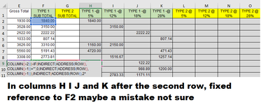
| 19 | IF B12="","" | IF B13="","" | IF B14="","" | IF B15="","" | ||||||||||||||||||||||
| 20 | I WILL TRY TO EXPLAIN MY PROBLEM AS SIMPLE AS POSSIBLE | IF J12 AND L12="" | IF N13="" | IF H14="" | IF J15="" | |||||||||||||||||||||
| 21 | If you change the amount in column B the difference amount in column Y should be zero only | THEN E12 AND F12 ="" | THAN G13="" | THAN D14="" | THAN E15="" | |||||||||||||||||||||
| 22 | I have given different formulas manually in columns D to K | AND D12=H12/2.5*100 | THEN D13=H13/2.5*100 | AND E14=J14/6*100 | AND D15=H15/2.5*100 | |||||||||||||||||||||
| 23 | There can be 15 different calculations for each amount entered in Column B | AND | AND | AND | AND | |||||||||||||||||||||
| 24 | The number of entries are in 1000's. I have been calculating it manually for each row using sort and filter options | G12=B12=D12 | E13=J13/6*100 | F14=L14/9*100 | F15=L15/9*100 | |||||||||||||||||||||
| 25 | I know it is possible to make it easy by giving a formula in the Row 4 from D4:K4 in each column and copy the formula till the last entry | AND | AND | AND | ||||||||||||||||||||||
| 26 | Due to lack of knowledge of multiple "IF", "AND" & "OR", I am finding it difficult to solve this. I would like to know and understand | F13=B13-H13-J13 | G14=B14-J14-L14 | G15=B15-D15-L15 | ||||||||||||||||||||||
| 27 | Since the last few weeks I have been trying but not able to solve it. I would really appreciate any help in solving this. | |||||||||||||||||||||||||
| 28 | Why don't you experts give it a try. If the solution is solved it will save me hours of work | ROW 16 | ROW 17 | ROW 18 | ||||||||||||||||||||||
| 29 | Please note that the amounts in columns H:P are also variables like in column B | IF B16="","" | IF B17="","" | IF B18="","" | ||||||||||||||||||||||
| 30 | Column C is an extension of my project and it will require to change only the references once I find a solution | IF J16="" | IF H17, J17,L17 AND N17<>"" | IF H18 AND L18 ="" | ||||||||||||||||||||||
| 31 | How it works | THEN F16="" | THEN D17=H16/2.5*100 | THEN D18="", F18="" | ||||||||||||||||||||||
| 32 | In columns H,J,L and N if there is amount in one cell only then it takes the amount from column B | AND D16=H16/2.5*100 | AND E17=J17/6*100 | AND E18=J18/6*100 | ||||||||||||||||||||||
| 33 | if there are amounts in any 2 cells in H, J, L and N then the first cell in D, E, F and G should be calculated from the corresponding column | AND | AND F17=L17/9*100 | AND G18=B18-E18 | ||||||||||||||||||||||
| 34 | and the second cell amount should be taken after deducting the total amount from the first calculated amount | F16= L16/9*100 | AND G17=B17-D17-E17-F17 | |||||||||||||||||||||||
| 35 | if there are amounts in 3 cells the again the first cell amount should be calculated from the corresponding column | AND | ||||||||||||||||||||||||
| 36 | the second amount also to be calculated from the corresponding column | G16=B16-D16-F16 | ||||||||||||||||||||||||
| 37 | and then in the third cell it should deduct the total amount from the first and second calculation amounts | |||||||||||||||||||||||||
| 38 | if there are amounts in all 4 cells then the first cell amount should be calculated from the corresponding column | |||||||||||||||||||||||||
| 39 | the second cell amount also to be calculated from the corresponding column | |||||||||||||||||||||||||
| 40 | the third cell amount also to be calculated from the corresponding column | |||||||||||||||||||||||||
| 41 | and the fourth cell it should deduct the total amount from the first, second and third calculated amounts | |||||||||||||||||||||||||
| 42 | ||||||||||||||||||||||||||
| 43 | ||||||||||||||||||||||||||
| 44 | ||||||||||||||||||||||||||
| 45 | ||||||||||||||||||||||||||
QUERY | ||||||||||||||||||||||||||
| Cell Formulas | ||
|---|---|---|
| Range | Formula | |
| D4 | D4 | =B4 |
| P4:P18 | P4 | =B4+C4-SUM(D4:O4) |
| Q4:Q18 | Q4 | =A4-SUM(D4:O4) |
| E5 | E5 | =B5 |
| F6 | F6 | =B6 |
| G7 | G7 | =B7 |
| D8,D15:D17,D11:D13 | D8 | =H8/2.5*100 |
| E8 | E8 | =B8-D8 |
| E9,E16:E17,E13:E14 | E9 | =J9/6*100 |
| G10 | G10 | =B10-F10 |
| F9 | F9 | =B9-E9 |
| F10,F17,F14:F15 | F10 | =L10/9*100 |
| F11 | F11 | =B11-D11 |
| G12 | G12 | =B12-D12 |
| F13 | F13 | =B13-D13-E13 |
| G14 | G14 | =B14-E14-F14 |
| G15 | G15 | =B15-D15-F15 |
| G16 | G16 | =B16-D16-E16 |
| A4:A17 | A4 | =SUM(C4:O4) |
| G17 | G17 | =B17-D17-E17-F17 |