Multiple Matches but only pulling 1st one

[CrashOD]

tried doing this codes looking for
C12 ' is the value i'm wanting to search for were they can be multi matches if there is i need B44-B46, D44-D46 have values in there
'SK Real Estate'!$U:$U ' is the location to look for the info to match to (C12)

B44 ' should show SK Real Estate'!$H:$H
'SK Real Estate'!$H:$H ' (Date) is the value i want returned if there is a value

B45 ' should show 'SK Real Estate'!$J:$J
'SK Real Estate'!$J:$J ' (Date) is the value i want returned if there is a value

B46 ' should show 'SK Real Estate'!$L:$L
'SK Real Estate'!$L:$L ' (Date) is the value i want returned if there is a value

D44 ' should show SK Real Estate'!$I:$I
'SK Real Estate'!$I:$I ' (Amount) is the value i want returned if there is a value

D45 ' should show 'SK Real Estate'!$K:$K
'SK Real Estate'!$K:$K ' (Amount) is the value i want returned if there is a value

D46 ' should show 'SK Real Estate'!$M:$M
'SK Real Estate'!$M:$M ' (Amount) is the value i want returned if there is a value

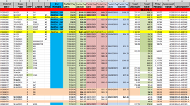
I tried the below codes with no luck. B44 & D44 get filled in but nothing more. on the picture below with the black boxes line 1170 in $U matches for the 2nd time witch should fill in B45 & d45 for 2nd payment.

=IF(ISNUMBER(MATCH('SK Real Estate'!$A:$U, $C$12)), MATCH($C$12('SK Real Estate'!$A:$U), ROW('SK Real Estate'!$A:$U)), "")

=INDEX('SK Real Estate'!$A:$U,MATCH(C12,'SK Real Estate'!$U:$U,0),8)

=IFERROR(INDEX('SK Real Estate'!$H:$H, SMALL(IF($C$12='SK Real Estate'!$U:$U, ROW('SK Real Estate'!$U:$U)-ROW('SK Real Estate'!$U)+1), ROW(1:1))),"" )


this picture shows were im pulling data from (this exact sheet in in the same workbook im looking to put code in. why i used 'SK Real Estate'! and not reference a workbook then sheet

the picture below is were im doing the code for B44:B46 & D44:d46. yes the total due is wrong for face changing code to pull the other amount on sheet should be

321.41​

327.97​

360.77​

Thanks so much for any help!

 

[KRice]

Given this:

MrExcel_20220603.xlsx
	H	I	J	K	L	M							T	U
1	PP Date1	PP Amt1	PP Date2	PP Amt2	PP Date3	PP Amt3								Description1
2
3														a1
4	1/2/2021	100	2/2/2021	101	3/2/2021	102								a2
5														b6
6	7/6/2021	109.33	8/2/2021	109.32	9/1/2021	110.01								b5
7														a5
8														c2
9														d1
10
11
12	map to B44	map to D44	map to B45	map to D45	map to B46	map to D46								match to C12
SK Real Estate

Try this for bringing over the payments and dates:

MrExcel_20220603.xlsx
	A	B	C	D
12		Description1	b5
42
43		dates		amts
44	Payment #1	7/6/2021		109.33
45	Payment #2	8/2/2021		109.32
46	Payment #3	9/1/2021		110.01
Tax Cert Form

Cell Formulas
Range	Formula
B44:B46	B44	=IFERROR(INDEX('SK Real Estate'!$H$3:$M$100,MATCH($C$12,'SK Real Estate'!$U$3:$U$100,0),2*ROWS(B$44:B44)-1),"" )
D44:D46	D44	=IFERROR(INDEX('SK Real Estate'!$H$3:$M$100,MATCH($C$12,'SK Real Estate'!$U$3:$U$100,0),2*ROWS(D$44:D44)),"" )

This assumes the match for C12 will be found on only one row in column U of the SK Real Estate sheet. If there are multiple rows where C12 matches, then more needs to be known to determine which row is of interest. If you have access to Excel 365 functions, this could be revised to used some updated functions.

 

[CrashOD]

Given this:

MrExcel_20220603.xlsx
	H	I	J	K	L	M							T	U
1	PP Date1	PP Amt1	PP Date2	PP Amt2	PP Date3	PP Amt3								Description1
2
3														a1
4	1/2/2021	100	2/2/2021	101	3/2/2021	102								a2
5														b6
6	7/6/2021	109.33	8/2/2021	109.32	9/1/2021	110.01								b5
7														a5
8														c2
9														d1
10
11
12	map to B44	map to D44	map to B45	map to D45	map to B46	map to D46								match to C12
SK Real Estate

Try this for bringing over the payments and dates:

MrExcel_20220603.xlsx
	A	B	C	D
12		Description1	b5
42
43		dates		amts
44	Payment #1	7/6/2021		109.33
45	Payment #2	8/2/2021		109.32
46	Payment #3	9/1/2021		110.01
Tax Cert Form

Cell Formulas
Range	Formula
B44:B46	B44	=IFERROR(INDEX('SK Real Estate'!$H$3:$M$100,MATCH($C$12,'SK Real Estate'!$U$3:$U$100,0),2*ROWS(B$44:B44)-1),"" )
D44:D46	D44	=IFERROR(INDEX('SK Real Estate'!$H$3:$M$100,MATCH($C$12,'SK Real Estate'!$U$3:$U$100,0),2*ROWS(D$44:D44)),"" )

This assumes the match for C12 will be found on only one row in column U of the SK Real Estate sheet. If there are multiple rows where C12 matches, then more needs to be known to determine which row is of interest. If you have access to Excel 365 functions, this could be revised to used some updated functions.

c12 is a parcel like 001-01-001-001 and it can be in a match for 3 times depending how many partial payments they made.

SCHOOL 2021	July/Aug	Sept/Oct	Nov/Dec
		Discount (-2%)	Face:	Penalty (+10%)
	PAID	$274.68	$280.29	$308.32
Date Paid:	8/16/2021		HomeStead	Assessed Value
			YES	9,900
	SHORT		$0.00
PAYMENT #1	7/26/21		93.43
PAYMENT #2	08/16/2021		93.43
PAYMENT #3	08/16/2021		93.43

 

[KRice]

I understand that...and that is what my formula does. It searches down SK Real Estate column U for the value in C12. When it finds the first match for that value, it returns up to three partial payments and the corresponding dates, placing them in B44:B46 and D44:D46 on the Tax Cert Form sheet. My question about the number of matches pertains to the red italicized text in the previous sentence: As one looks down column U on the SK Real Estate sheets, will there be only one match found in that column? If there are multiple matches, the formula will use only the first match.

 

[CrashOD]

I understand that...and that is what my formula does. It searches down SK Real Estate column U for the value in C12. When it finds the first match for that value, it returns up to three partial payments and the corresponding dates, placing them in B44:B46 and D44:D46 on the Tax Cert Form sheet. My question about the number of matches pertains to the red italicized text in the previous sentence: As one looks down column U on the SK Real Estate sheets, will there be only one match found in that column? If there are multiple matches, the formula will use only the first match.

Yes if partial payment c12 (PARCEL)-(column U)can be in there up to 3 times, one for each payment made

 

[KRice]

I don't understand that answer. In your first post, you don't show cell C12 on the Tax Cert Form. I'm assuming it is supposed to match cell U1170 on the SK Real Estate sheet...that cell is partially blacked out, so I can't see the full number, but I know it begins with 01 and ends with 004-149, and some middle portion--let's say it's xxx--is blacked out. I don't see any other item in column U that is 01xxx004-149, so I assume there will be only one row that is of interest. In your example, you show two partial payments on row 1170. My formula would pull all of the partial payments on that same row 1170.

Have you tried my formula? Does it not return the expected values?

 

[CrashOD]

hope this helps.

 

[KRice]

Thank you...that does help. If you go back to my first post on this thread:

This assumes the match for C12 will be found on only one row in column U of the SK Real Estate sheet. If there are multiple rows where C12 matches, then more needs to be known to determine which row is of interest. If you have access to Excel 365 functions, this could be revised to used some updated functions.

The answer is that my assumption was not correct. The match for C12 can indeed be found on multiple rows in column U of the SK Real Estate Sheet...so more information is needed to determine which row is of interest. In your most recent post (#7), you show several examples where the same value is found on multiple rows in column U. Unfortunately, this is fundamentally different from what you presented in post #1, where every value in column U is unique...there are no instances shown of multiple matches. However, in your most recent post, it appears that the first match of any potential multiple match sets seems to contain all of the partial payments aggregated on the same row. If that is true--and that is a critical piece of information--then the formula I suggested in post #2 should work fine because it operates on the first match. So I will once again ask if you have evaluated the formula to determine if it produces the results you expect?

 

[CrashOD]

Automated 2022 Tax Certification Form.xlsm
	A	B	C	D	E
38	SCHOOL 2021		July/Aug	Sept/Oct	Nov/Dec
39			Discount (-2%)	Face:	Penalty (+10%)
40		PAID	$166.36	$169.76	$186.74
41	Date Paid:	01/00/1900		HomeStead	Assessed Value
42				NO	4,700
43		PARTIALS	DATE	$113.16	<- SHORT IN FACE
44		PAYMENT #1	7/20/2021	$56.60	FACE
45		PAYMENT #2	01/00/1900	$0.00	FACE
46		PAYMENT #3	01/00/1900	$0.00	FACE
Tax Cert Form 2022-2021 (2)

Cell Formulas
Range	Formula
C40	C40	=INDEX('SK Real Estate'!$A:$AK,MATCH(C12,'SK Real Estate'!$U:$U,0),31)
D40	D40	=INDEX('SK Real Estate'!$A:$AK,MATCH(C12,'SK Real Estate'!$U:$U,0),32)
E40	E40	=INDEX('SK Real Estate'!$A:$AK,MATCH(C12,'SK Real Estate'!$U:$U,0),33)
B40	B40	=IF(B41="","UNPAID",IF(B41="EXONERATED", "PER COUNTY", "PAID"))
B41	B41	=IF(D40>=D43, C46, INDEX('SK Real Estate'!$A:$U,MATCH(C12,'SK Real Estate'!$U:$U,0),3))
E42	E42	=INDEX('SK Real Estate'!$A:$U,MATCH(C12,'SK Real Estate'!$U:$U,0),20)
D42	D42	=INDEX('SK Real Estate'!$A:$AI,MATCH(C12,'SK Real Estate'!$U:$U,0),35)
D43	D43	=IF(D44="","",IF((D44+D45+D46)>=D40,0,(D40-D44-D45-D46)))
C44:C46	C44	=IFERROR(INDEX('SK Real Estate'!$H$3:$M$100,MATCH($C$12,'SK Real Estate'!$U$3:$U$100,0),2*ROWS(C$44:C44)-1),"" )
D44:D46	D44	=IFERROR(INDEX('SK Real Estate'!$H$3:$M$100,MATCH($C$12,'SK Real Estate'!$U$3:$U$100,0),2*ROWS(D$44:D44)),"" )
E44	E44	=IF(C44="","", "FACE")
E45:E46	E45	=IF(C45="","",IF( D45<=D44, "FACE", IF(D44>D45, "PENALTY")))

Named Ranges
Name	Refers To	Cells
'SK Real Estate'!CSV49XLS_7	='SK Real Estate'!$A$3:$AG$4224	B41, D42:E42, C40:E40

Works but when no data fills in with the weird date and a 0 needing it to show nothing if nothing but that is a great help thanks!

 

[KRice]

Yes...that's why I was trying to determine if you had access to Excel 365 functions. If you click on an empty cell and begin typing =FIILTER does Excel recognize the filter function? If not, then to deal with the cases where there are blanks, some additional changes will be needed to the formula, but if you have 365, the solution to this is simpler.