Multiple search criteria within the same spreadsheet

[Lore0818]

Hello all,
I'm sure you can tell I'm a newbie to excel by the thread I'm posting. I've read so many posts on multiple searches, however I couldn't find any that fits what I'm looking for. Maybe I'm tired and just can't see or think outside the box.
It's simple what I'm trying to do and would be soooooo helpful.

I'm trying to look up multiple zip codes at the same time in one spreadsheet.
I have found online where I can group all the zip codes within a 25 mile radius of a specific location.
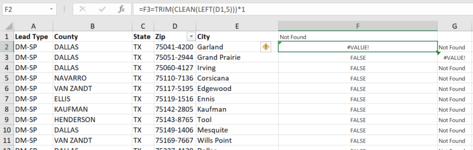
Now, I'm trying to lookup all those 20+ zip codes on a spreadsheet which contains client info including their zip code (in a separate column)
Column I containes the zip codes I'm trying to search in the spreadsheet of about 2000+ rows of data.

Thank you advance for any help.

 

[Saba Sabaratnam]

Try this formula. Copy this formula as it is in F2 and copy it down.

=XLOOKUP(LEFT(TRIM(D1),5)*1,$J$3:$J$57,$J$3:$J$57,"Not Found")

if it does not work, copy a data point (say D2) as text so that I can see the structure of your data.

Kind regards

Saba

 

[Lore0818]

I'm sorry, I don't understand what you're asking me to do.
Is this what you're asking?
I promise I won't get offended if you give me instructions as if I was 4 years old.

Lead Type	County	State	Zip	City	Not Found
DM-SP	DALLAS	TX	75041-4200	Garland	#VALUE!​
DM-SP	DALLAS	TX	75051-2944	Grand Prairie	Not Found
DM-SP	DALLAS	TX	75060-4127	Irving	Not Found
DM-SP	NAVARRO	TX	75110-7136	Corsicana	Not Found
DM-SP	VAN ZANDT	TX	75117-5195	Edgewood	Not Found

 

[Saba Sabaratnam]

no problem


You could try this approach.

Enter the following formula in F2 and copy it down to extract first five digits of your code and turn it to number.

=TRIM(CLEAN(LEFT(D1,5)))*1

Then this formula in G2 and copy it down.

=XLOOKUP(F1,$K$3:$K$57,$K$3:$K$57,"Not Found")

Kind regards

Saba

 

[Lore0818]

These are my results.

 

[Saba Sabaratnam]

Try this formula by coping in F1 as it is.

=IF(SUM(IF(ISNUMBER(SEARCH(IF($I$3:$I$57<>"",$I$3:$I$57,NA()),D1,1)),SEARCH(IF($I$3:$I$57<>"",$I$3:$I$57,NA()),D1,1),0))>0,LEFT(D1,5),"Not Found")

Then copy F1 and paste the formula from f2 to the last row of data of column F.

Kind regards

Saba

 

[Lore0818]

These were my results "not found" all the way down the F column. I even checked every so many rows all the way down to make sure it had been copied all the way through.

 

[Saba Sabaratnam]

It is referencing to wrong lookup reference.

Use this formula .

==IF(SUM(IF(ISNUMBER(SEARCH(IF($J$3:$J$57<>"",$J$3:$J$57,NA()),D1,1)),SEARCH(IF($J$3:$J$57<>"",$J$3:$J$57,NA()),D1,1),0))>0,LEFT(D1,5),"Not Found")

Kind regards

Saba

 

[Lore0818]

if won't let me use 2 equal signs..... ==
So I took one out and it displays 'not found'

 

[Saba Sabaratnam]

Only single = sign please.

Include 75041 in J3 (replace 76511 with this number) to see if the formula produces 75041 or
"Not found" result.

Also can you please confirm that you have office 365?

Kind regards

Saba

 

[Lore0818]

Yes...Yes...YES!!!!!
The last formula worked. I created a filter in column F (which I should've done from the beggining) and it displayed what I was looking for.
Thank you SOOOOOOOO much Saba.