My formula is not displaying the result.

[jjk1]

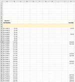
My formula is not displaying the result. It seems like it is identifying the result, but not displaying it in the cell where this formula resides.

=IFERROR(INDEX($J1, MATCH(MIN(IF(ISNUMBER($D:$D), MATCH($D:$D, $D:$D, 0))), MATCH($D:$D, $D:$D, 0), 0)), "")

What its suppose to do:
Search column D.
This first time a value appears in column D, identify the number that appears in column J of the same row, and display it in column K of the same row where the formula is.
In column D, any instances where the value appears multiple times, it is only the first occurrence that should be displayed.

(this formula searches "numbers" in column D. Once I can get this to work, then i need one that searches through "text" in column D) and works the same way.

Thank you

 

[ExceLoki]

which version of excel are you using? this helps when trying to find a solution. you can update in your profile.

 

[AhoyNC]

Your INDEX syntax is wrong.
If you are just looking for the first number in column D try changing your INDEX formula to:
INDEX(J:J,MATCH(TRUE,ISNUMBER(D:D),0)

Also, it is not the best idea to reference whole columns. If your data won't go below say row 10000 and you have headers in row one then reduce your range to J1:J10000.

As pointed out by ExceLoki it helps if we know what version of Excel you are using.

 

[jjk1]

I updated my prole. Its excel 2019 in windows.

I tried the formula y recommended and it does not work. It returns #N/A.

If I was not clear, column D and each cell will have a number. The column will have a variety of numbers. So for the if the number is the first occurrence within column D of that number, then I want it to display the value in the same row from column J.

Please let me know if further clarification is needed. thank you.

 

[jjk1]

which version of excel are you using? this helps when trying to find a solution. you can update in your profile.

excel 2019 windows version.

 

[jjk1]

Your INDEX syntax is wrong.
If you are just looking for the first number in column D try changing your INDEX formula to:
INDEX(J:J,MATCH(TRUE,ISNUMBER(D:D),0)

Also, it is not the best idea to reference whole columns. If your data won't go below say row 10000 and you have headers in row one then reduce your range to J1:J10000.

As pointed out by ExceLoki it helps if we know what version of Excel you are using.

I tried your formula but it did not work. it returns #N/A

 

[AhoyNC]

It would help if you would post a small sample and the expected results.
Are you looking for something like this?

Book2
	D	E					J	K
2	6						10	10
3	2						20	20
4	10						30	30
5	6						40	10
6	45						50	50
7	1						60	60
8	45						70	50
9	6						80	10
Sheet1

Cell Formulas
Range	Formula
K2:K9	K2	=INDEX($J$2:$J$9,MATCH($D2,$D$2:$D$9,0))

 

[jjk1]

In my sample image the formula should produce the sample results as they appear in column K.
In your example 6 appears 3 times, but it should only produce a result the first time it appears in column D. Also, 45 appears twice, it should only produce a result the first time i appears in column D.

 

[AhoyNC]

Try:

Book2
	A	B	C	D	E					J	K
10	Random
11	Ref Number										Formula
12
13
14	EF1239876	$3.00									$3.00
15	EF1239876	$4.00
16	EF1239876	$5.00
17	EF1239833	$6.00									$6.00
18	EF1239833	$7.00
19	EF1239833	$8.00
20	EF1239833	$9.00
21	EF1239890	$10.00									$10.00
22	EF1239897	$11.00									$11.00
23	EF1239897	$12.00
24	EF1239897	$13.00
25	EF1239897	$14.00
26	EF1239897	$15.00
27	EF1239904	$16.00									$16.00
28	EF1239911	$17.00									$17.00
29	EF1239911	$18.00
30	EF1239911	$19.00
31	EF1239918	$20.00									$20.00
32	EF1239925	$21.00									$21.00
33	EF1239925	$22.00
34	EF1239925	$23.00
35	EF1239925	$24.00
36	EF1239925	$25.00
37	EF1239925	$26.00
38	EF1239332	$27.00									$27.00
39	EF1239939	$28.00									$28.00
40	EF1239946	$29.00									$29.00
41	EF1239953	$30.00									$30.00
Sheet2

Cell Formulas
Range	Formula
K14:K41	K14	=IF(COUNTIF($A$14:$A14,A14)=1,INDEX($B$14:$B$41,MATCH($B14,$B$14:$B14,0)),"")

 

[jjk1]

Thank you it works perfect!!
Now I have add a layer of complexity. I need to use our formula to pull out the result from within a text string in my formula. The result would appear in column "K" for each row as you did above.

The formula below works for what I need, however I need the conditions that are in the formula you wrote to apply the below formula:

IFERROR(IF(IF(MID(A15,3,1)="b",IF(AND(MID(A15,47,1)="-",(MID(A15,29,18)/100)<>0),"+",IF(AND(MID(A15,47,1)="+",(MID(A15,29,18)/100)<>0),"-","")),"")="+",IF(MID(A14,3,1)="a",MID(A14,181,18)/100,"")+IF(MID(A15,3,1)="b",MID(A15,29,18)/100,"")*1,IF(MID(A14,3,1)="a",MID(A14,181,18)/100,"")+IF(MID(A15,3,1)="b",MID(A15,29,18)/100,"")*-1),"")

Thank you!