Need a formula that will return true if one value is closer to zero than another

[MagicMoogle]

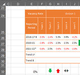
Hi everyone, on the attached image I need a formula for rows 29 and 30 that will return the arrows in row 32 depending on which value is closest to zero, syntax for the "trend LY" row would be something like this (using column F as an example):

if F28 is closer to E32 than F27, return G32, if F28 is further away from E32 than F27, return H32, if F28=F27, return I32.

Then for the "Trend B" it would be the same, except F26 would be the comparator instead of F27. I know the direction of the arrows might seem counterintuitive, but the upwards/downwards position is about the variance from zero rather than the actual numbers themselves, so cell F29 would be a red upwards arrow because although mathematically 5.6% (F28) is a lower value than -1.8% (F27), its variance from zero is greater.

Unfortunately I haven't been able to find any operators for "closer than" or "further away" so this might be quite complex. I've been playing around with nested if statements for days but can't seem to get over this hump. Any help anyone could provide would be fantastic.

Thanks!

 

[etaf]

would ABS() help, so that eliminates negative v positive

so

if F28 is closer to E32 than F27, return G32, if F28 is further away from E32 than F27, return H32, if F28=F27, return I32.

Does this answer the first part of question ?
=IF( F28=F27 , I32 , IF ( (ABS(F28)-E32 ) < (ABS(F27)-E32 ) , F27 , H32 ))


Note: Images are difficult to see , and also requires that I input all the data myself, which is very time consuming.

A SMALL sample spreadsheet, around 10-20 rows, would help a lot here, with all sensitive data removed, and expected results mocked up and manually entered, with a few notes of explanation.

MrExcel has a tool called “XL2BB” that lets you post samples of your data and will allow us to copy/paste your sample data into our Excel spreadsheets, saving a lot of time.

XL2BB - Excel Range to BBCode

Excel 'mini-sheet' in messages - XL2BB Although experts prefer to read your description and question instead of working in your actual file to solve your problem, there are times that it is difficult to explain an issue without providing actual...

www.mrexcel.com

You can also test to see if it works ok, in the "Test Here" forum.

Test Here

Use this forum to test your signature, learn bbcode, smilies, XL2BB, etc. Threads in this forum are automatically deleted after no replies for seven (7) days

www.mrexcel.com

OR if you cannot get XL2BB to work, or have restrictions on your PC , then put the sample spreadsheet onto a share
I only tend to goto OneDrive, Dropbox or google docs , as I'm never certain of other random share sites and possible virus.
Please make sure you have a representative data sample and also that the data has been desensitised, remember this site is open to anyone with internet access to see - so any sensitive / personal data should be removed

 

[MagicMoogle]

would ABS() help, so that eliminates negative v positive

so


Does this answer the first part of question ?
=IF( F28=F27 , I32 , IF ( (ABS(F28)-E32 ) < (ABS(F27)-E32 ) , F27 , H32 ))


Note: Images are difficult to see , and also requires that I input all the data myself, which is very time consuming.

A SMALL sample spreadsheet, around 10-20 rows, would help a lot here, with all sensitive data removed, and expected results mocked up and manually entered, with a few notes of explanation.

MrExcel has a tool called “XL2BB” that lets you post samples of your data and will allow us to copy/paste your sample data into our Excel spreadsheets, saving a lot of time.

XL2BB - Excel Range to BBCode

Excel 'mini-sheet' in messages - XL2BB Although experts prefer to read your description and question instead of working in your actual file to solve your problem, there are times that it is difficult to explain an issue without providing actual...

www.mrexcel.com

You can also test to see if it works ok, in the "Test Here" forum.

Test Here

Use this forum to test your signature, learn bbcode, smilies, XL2BB, etc. Threads in this forum are automatically deleted after no replies for seven (7) days

www.mrexcel.com

OR if you cannot get XL2BB to work, or have restrictions on your PC , then put the sample spreadsheet onto a share
I only tend to goto OneDrive, Dropbox or google docs , as I'm never certain of other random share sites and possible virus.
Please make sure you have a representative data sample and also that the data has been desensitised, remember this site is open to anyone with internet access to see - so any sensitive / personal data should be removed

Etaf thank you so much your initial formula using ABS has solved my problem! I hadn't considered this approach at all. Many thanks again.

 

[etaf]

you are welcome