Hey everyone! I am pulling out my hair and finally decided I just needed to ask for help somewhere. Apparently, I know just enough to be dangerous... 
I am creating a dashboard with multiple locations that I need to roll up into one summary page. Each location is on a separate worksheet. The data is laid out with the rows representing weeks and the columns representing service times. There are multiple categories for each service time and not every location has the same service time. I can write an array INDEX MATCH MATCH formula to pull one location at a time, but if I try to add them all together, it breaks. I tried SUMIFS, but couldn't make that work either.
What I really want is to add together all the matching cells from each sheet, but if ALL matching cells are blank, I want the result to be a blank, as well. I don't want a bunch of zeros for future weeks.
In the end, after not being able to make either SUMIFS or INDEX MATCH MATCH work, I resorted to SUMPRODUCT, and hoped that it wouldn't slow down my workbook too much. Well, it did. Now as I am trying to populate the historical data in each location, there is literally a 5-10 second lag after inputting a cell before it will move to the next cell. I broke the workbook, even though my summary page is displayed what I want.
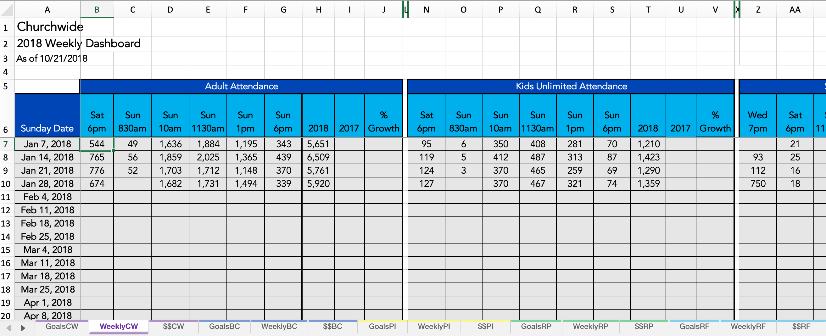
Here is what my summary page looks like currently, with my SUMPRODUCT formula (this works for me):
My SUMPRODUCT formula is as follows (I have multiple helper cells in row 4 with the names of the headers with white text that I used when I thought I could make INDEX MATCH MATCH work):
=IF(SUMPRODUCT((WeeklyBC!$A$7:$A$60=WeeklyCW!$A7)*(WeeklyBC!$B$6:$DT$6=WeeklyCW!B$6)*(WeeklyBC!$B$4:$DT$4=WeeklyCW!B$4),WeeklyBC!$B$7:$DT$60)+SUMPRODUCT((WeeklyPI!$A$7:$A$60=WeeklyCW!$A7)*(WeeklyPI!$B$6:$DB$6=WeeklyCW!B$6)*(WeeklyPI!$B$4:$DB$4=WeeklyCW!B$4),WeeklyPI!$B$7:$DB$60)+SUMPRODUCT((WeeklyRP!$A$7:$A$60=WeeklyCW!$A7)*(WeeklyRP!$B$6:$CT$6=WeeklyCW!B$6)*(WeeklyRP!$B$4:$CT$4=WeeklyCW!B$4),WeeklyRP!$B$7:$CT$60)+SUMPRODUCT((WeeklyRF!$A$7:$A$60=WeeklyCW!$A7)*(WeeklyRF!$B$6:$DL$6=WeeklyCW!B$6)*(WeeklyRF!$B$4:$DL$4=WeeklyCW!B$4),WeeklyRF!$B$7:$DL$60)+SUMPRODUCT((WeeklySA!$A$7:$A$60=WeeklyCW!$A7)*(WeeklySA!$B$6:$CT$6=WeeklyCW!B$6)*(WeeklySA!$B$4:$CT$4=WeeklyCW!B$4),WeeklySA!$B$7:$CT$60)+SUMPRODUCT((WeeklyWS!$A$7:$A$60=WeeklyCW!$A7)*(WeeklyWS!$B$6:$DJ$6=WeeklyCW!B$6)*(WeeklyWS!$B$4:$DJ$4=WeeklyCW!B$4),WeeklyWS!$B$7:$DJ$60)=0,"",SUMPRODUCT((WeeklyBC!$A$7:$A$60=WeeklyCW!$A7)*(WeeklyBC!$B$6:$DT$6=WeeklyCW!B$6)*(WeeklyBC!$B$4:$DT$4=WeeklyCW!B$4),WeeklyBC!$B$7:$DT$60)+SUMPRODUCT((WeeklyPI!$A$7:$A$60=WeeklyCW!$A7)*(WeeklyPI!$B$6:$DB$6=WeeklyCW!B$6)*(WeeklyPI!$B$4:$DB$4=WeeklyCW!B$4),WeeklyPI!$B$7:$DB$60)+SUMPRODUCT((WeeklyRP!$A$7:$A$60=WeeklyCW!$A7)*(WeeklyRP!$B$6:$CT$6=WeeklyCW!B$6)*(WeeklyRP!$B$4:$CT$4=WeeklyCW!B$4),WeeklyRP!$B$7:$CT$60)+SUMPRODUCT((WeeklyRF!$A$7:$A$60=WeeklyCW!$A7)*(WeeklyRF!$B$6:$DL$6=WeeklyCW!B$6)*(WeeklyRF!$B$4:$DL$4=WeeklyCW!B$4),WeeklyRF!$B$7:$DL$60)+SUMPRODUCT((WeeklySA!$A$7:$A$60=WeeklyCW!$A7)*(WeeklySA!$B$6:$CT$6=WeeklyCW!B$6)*(WeeklySA!$B$4:$CT$4=WeeklyCW!B$4),WeeklySA!$B$7:$CT$60)+SUMPRODUCT((WeeklyWS!$A$7:$A$60=WeeklyCW!$A7)*(WeeklyWS!$B$6:$DJ$6=WeeklyCW!B$6)*(WeeklyWS!$B$4:$DJ$4=WeeklyCW!B$4),WeeklyWS!$B$7:$DJ$60))
The INDEX MATCH MATCH formula I was trying to expand upon was: {=IFERROR(INDEX(WeeklyBC!$B$7:$DT$60,MATCH(WeeklyCW!$A7,WeeklyBC!$A$6:$A60,0),MATCH(1,(WeeklyCW!B$6=WeeklyBC!$B$6:$DT$6)*(WeeklyCW!B$4=WeeklyBC!$B$4:$DT$4),0)),"")}
I was hoping to just add a bunch of those together from each sheet, but it keeps breaking on me when there is no match on one of the sheets. It works great if it finds a match on all sheets, but otherwise, it breaks.
For example, both the BC and PI sheets have a 10am service under adult attendance, so this works fine: {=IFERROR(INDEX(WeeklyBC!$B$7:$DT$60,MATCH(WeeklyCW!$A7,WeeklyBC!$A$6:$A60,0),MATCH(1,(WeeklyCW!D$6=WeeklyBC!$B$6:$DT$6)*(WeeklyCW!D$4=WeeklyBC!$B$4:$DT$4),0)),"")+IFERROR(INDEX(WeeklyPI!$B$7:$DB$60,MATCH(WeeklyCW!$A7,WeeklyPI!$A$6:$A60,0),MATCH(1,(WeeklyCW!D$6=WeeklyPI!$B$6:$DB$6)*(WeeklyCW!D$4=WeeklyPI!$B$4:$DB$4),0)),"")}.
However, it returns #VALUE for the Sat 6pm service, because PI doesn't have that. And, if I put it in a future week where there is no data at all, it returns 0.
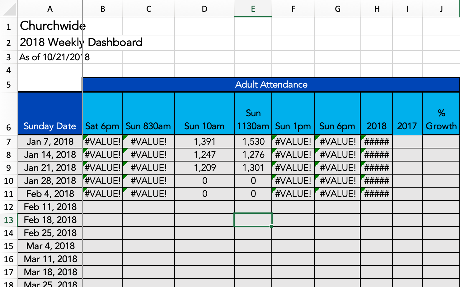
I just want it to ignore errors (no match) and return a blank if all the matching cells are blank. I have tried wrapping the entire thing in not blank formulas, but they don't seem to work, so that must be where I'm going wrong. I think at some point I tried to SUMIF or SUMIFS the whole thing together, as well, but I just can't seem to put it all together...
I hope that makes sense. Please let me know if there is more data sampling needed, etc. and I appreciate any assistance!ray:
I am creating a dashboard with multiple locations that I need to roll up into one summary page. Each location is on a separate worksheet. The data is laid out with the rows representing weeks and the columns representing service times. There are multiple categories for each service time and not every location has the same service time. I can write an array INDEX MATCH MATCH formula to pull one location at a time, but if I try to add them all together, it breaks. I tried SUMIFS, but couldn't make that work either.
What I really want is to add together all the matching cells from each sheet, but if ALL matching cells are blank, I want the result to be a blank, as well. I don't want a bunch of zeros for future weeks.
In the end, after not being able to make either SUMIFS or INDEX MATCH MATCH work, I resorted to SUMPRODUCT, and hoped that it wouldn't slow down my workbook too much. Well, it did. Now as I am trying to populate the historical data in each location, there is literally a 5-10 second lag after inputting a cell before it will move to the next cell. I broke the workbook, even though my summary page is displayed what I want.
Here is what my summary page looks like currently, with my SUMPRODUCT formula (this works for me):
My SUMPRODUCT formula is as follows (I have multiple helper cells in row 4 with the names of the headers with white text that I used when I thought I could make INDEX MATCH MATCH work):
=IF(SUMPRODUCT((WeeklyBC!$A$7:$A$60=WeeklyCW!$A7)*(WeeklyBC!$B$6:$DT$6=WeeklyCW!B$6)*(WeeklyBC!$B$4:$DT$4=WeeklyCW!B$4),WeeklyBC!$B$7:$DT$60)+SUMPRODUCT((WeeklyPI!$A$7:$A$60=WeeklyCW!$A7)*(WeeklyPI!$B$6:$DB$6=WeeklyCW!B$6)*(WeeklyPI!$B$4:$DB$4=WeeklyCW!B$4),WeeklyPI!$B$7:$DB$60)+SUMPRODUCT((WeeklyRP!$A$7:$A$60=WeeklyCW!$A7)*(WeeklyRP!$B$6:$CT$6=WeeklyCW!B$6)*(WeeklyRP!$B$4:$CT$4=WeeklyCW!B$4),WeeklyRP!$B$7:$CT$60)+SUMPRODUCT((WeeklyRF!$A$7:$A$60=WeeklyCW!$A7)*(WeeklyRF!$B$6:$DL$6=WeeklyCW!B$6)*(WeeklyRF!$B$4:$DL$4=WeeklyCW!B$4),WeeklyRF!$B$7:$DL$60)+SUMPRODUCT((WeeklySA!$A$7:$A$60=WeeklyCW!$A7)*(WeeklySA!$B$6:$CT$6=WeeklyCW!B$6)*(WeeklySA!$B$4:$CT$4=WeeklyCW!B$4),WeeklySA!$B$7:$CT$60)+SUMPRODUCT((WeeklyWS!$A$7:$A$60=WeeklyCW!$A7)*(WeeklyWS!$B$6:$DJ$6=WeeklyCW!B$6)*(WeeklyWS!$B$4:$DJ$4=WeeklyCW!B$4),WeeklyWS!$B$7:$DJ$60)=0,"",SUMPRODUCT((WeeklyBC!$A$7:$A$60=WeeklyCW!$A7)*(WeeklyBC!$B$6:$DT$6=WeeklyCW!B$6)*(WeeklyBC!$B$4:$DT$4=WeeklyCW!B$4),WeeklyBC!$B$7:$DT$60)+SUMPRODUCT((WeeklyPI!$A$7:$A$60=WeeklyCW!$A7)*(WeeklyPI!$B$6:$DB$6=WeeklyCW!B$6)*(WeeklyPI!$B$4:$DB$4=WeeklyCW!B$4),WeeklyPI!$B$7:$DB$60)+SUMPRODUCT((WeeklyRP!$A$7:$A$60=WeeklyCW!$A7)*(WeeklyRP!$B$6:$CT$6=WeeklyCW!B$6)*(WeeklyRP!$B$4:$CT$4=WeeklyCW!B$4),WeeklyRP!$B$7:$CT$60)+SUMPRODUCT((WeeklyRF!$A$7:$A$60=WeeklyCW!$A7)*(WeeklyRF!$B$6:$DL$6=WeeklyCW!B$6)*(WeeklyRF!$B$4:$DL$4=WeeklyCW!B$4),WeeklyRF!$B$7:$DL$60)+SUMPRODUCT((WeeklySA!$A$7:$A$60=WeeklyCW!$A7)*(WeeklySA!$B$6:$CT$6=WeeklyCW!B$6)*(WeeklySA!$B$4:$CT$4=WeeklyCW!B$4),WeeklySA!$B$7:$CT$60)+SUMPRODUCT((WeeklyWS!$A$7:$A$60=WeeklyCW!$A7)*(WeeklyWS!$B$6:$DJ$6=WeeklyCW!B$6)*(WeeklyWS!$B$4:$DJ$4=WeeklyCW!B$4),WeeklyWS!$B$7:$DJ$60))
The INDEX MATCH MATCH formula I was trying to expand upon was: {=IFERROR(INDEX(WeeklyBC!$B$7:$DT$60,MATCH(WeeklyCW!$A7,WeeklyBC!$A$6:$A60,0),MATCH(1,(WeeklyCW!B$6=WeeklyBC!$B$6:$DT$6)*(WeeklyCW!B$4=WeeklyBC!$B$4:$DT$4),0)),"")}
I was hoping to just add a bunch of those together from each sheet, but it keeps breaking on me when there is no match on one of the sheets. It works great if it finds a match on all sheets, but otherwise, it breaks.
For example, both the BC and PI sheets have a 10am service under adult attendance, so this works fine: {=IFERROR(INDEX(WeeklyBC!$B$7:$DT$60,MATCH(WeeklyCW!$A7,WeeklyBC!$A$6:$A60,0),MATCH(1,(WeeklyCW!D$6=WeeklyBC!$B$6:$DT$6)*(WeeklyCW!D$4=WeeklyBC!$B$4:$DT$4),0)),"")+IFERROR(INDEX(WeeklyPI!$B$7:$DB$60,MATCH(WeeklyCW!$A7,WeeklyPI!$A$6:$A60,0),MATCH(1,(WeeklyCW!D$6=WeeklyPI!$B$6:$DB$6)*(WeeklyCW!D$4=WeeklyPI!$B$4:$DB$4),0)),"")}.
However, it returns #VALUE for the Sat 6pm service, because PI doesn't have that. And, if I put it in a future week where there is no data at all, it returns 0.
I just want it to ignore errors (no match) and return a blank if all the matching cells are blank. I have tried wrapping the entire thing in not blank formulas, but they don't seem to work, so that must be where I'm going wrong. I think at some point I tried to SUMIF or SUMIFS the whole thing together, as well, but I just can't seem to put it all together...
I hope that makes sense. Please let me know if there is more data sampling needed, etc. and I appreciate any assistance!
ray:


